Loop-dependent entangling holonomies in localized topological quartets

1 Introduction

An isolated four-state manifold can admit a pointwise two-qubit description and still return from a closed loop by a nonlocal gate. The same quartet may be almost local on one loop and entangling on another. In the BHZ ribbon studied below, co-rotating and counter-rotating edge-field loops act on the same helical quartet, but only the counter-rotating loop leaves the extracted local subgroup by an order-one amount.

Standard reduced Berry data do not resolve this difference. Chern numbers, determinant phases, and Wilson-loop eigenphases record phases or spectra of the loop operator. The question asked here is different. In the extracted local frame, can the microscopic holonomy be written as two independent single-qubit actions? Nearly identical eigenphase data can hide different gate classes, and a large Berry phase can occur on an almost local loop. What matters is whether the holonomy stays inside the extracted local subgroup.

The three benchmarks used below are standard settings in which localized four-state manifolds arise. The Bernevig-Hughes-Zhang (BHZ) model describes a two-dimensional quantum spin Hall insulator and supplies a helical pair on each open boundary [1]. The spinful Su-Schrieffer-Heeger (SSH) chain is a one-dimensional dimerized system whose two end modes are doubled by spin [2]. The Benalcazar-Bernevig-Hughes (BBH) quadrupole model is a two-dimensional higher-order topological insulator (HOTI) with states localized at its four corners [3]. In this paper, a quartet is the spectrally isolated four-dimensional subspace formed by these boundary states.

Each model has two independently tunable periodic angles associated with boundary or corner fields. Their parameter space is a control torus. A loop is a closed path on this torus, and the Wilczek-Zee holonomy is the unitary parallel transport of the isolated quartet generated by the projected Berry connection. Throughout the paper, “local” refers to a specified $2\; \times \; 2$ subsystem structure inside the quartet; it does not mean spatial locality in the microscopic lattice Hamiltonian. The physical origin of the two factors is stated at the beginning of each model section.

The two-qubit language is the smallest instance of a more general subsystem-reduction problem. If an isolated low-energy multiplet carries pointwise labels of dimensions $(d_1,\dots ,d_r)$, the relevant local structure group is not the full $\mathrm{\text{U}}(D)$, with $D\; ={\prod }_{\alpha =1}^r{d}_{\alpha }$, but the embedded product subgroup [4]

$$G_{\mathbf{\text{𝐝}}}:=\; Im\left[\underset{\alpha =1}{\overset{r}{\prod }}\mathrm{\text{U}}(d_{\alpha })\to \mathrm{\text{U}}(D)\right]\subset \mathrm{\text{U}}(D),(V_1,\dots ,V_r)\mapsto V_1\otimes \cdots \; \otimes V_r.$$

(1.1)

A loop holonomy may preserve these labels point by point and still leave $G_{\mathbf{\text{𝐝}}}$ after parallel transport around a closed path. In that case the loop glues the extracted product structure by an entangling element, or more generally by an element that is nonlocal with respect to the chosen factorization. The real codimension of $G_{\mathbf{\text{𝐝}}}$ inside $\mathrm{\text{U}}(D)$ is $D^2-{\sum }_{\alpha =1}^r{d}_{\alpha }^2+\; (r\; -\; 1)$. It is positive for every nontrivial factorization. Components transverse to the local algebra are therefore expected unless they are excluded by symmetry, locality, or the choice of controls. The rank-four case $\mathbf{\text{𝐝}}=\; (2,2)$ is the smallest setting in which this can be examined explicitly and related to standard two-qubit gate classes.

Geometric phases and their non-Abelian generalization are standard [5, 6]. Holonomies as quantum gates are also well known [7, 8]. Wilson-loop and eigenphase diagnostics are widely used in topological band theory and materials calculations [9–13], and non-Abelian Wilson loops are beginning to be measured directly [14, 15]. The question considered here is narrower. Once a local two-qubit structure has been extracted from a spectrally isolated quartet, does the loop holonomy remain in the corresponding local subgroup, and if not, what gate class does it realize?

The geometric input is the connection on the isolated quartet bundle. Its curvature is the non-Abelian Berry curvature of that bundle, not the Riemannian curvature of the control torus. The control torus may be flat in the coordinates $({𝜃}_1,{𝜃}_2)$ while the quartet connection still has nonzero curvature. The extra structure needed here is the extracted local subgroup. Once the local frame has been fixed, both the loop holonomy and, infinitesimally, the curvature can be decomposed into components tangent to ${𝔤}_{\mathbf{\text{𝐝}}}$ and components transverse to it. The transverse component is the part that can drive the holonomy outside $\mathrm{\text{U}}(2)\; \otimes \mathrm{\text{U}}(2)$.

This question matters in condensed-matter settings where localized boundary multiplets are used as effective qubits or as adiabatic control manifolds. Helical edge states, end modes, and corner multiplets are often described by low-energy labels that factor point by point in parameter space. These labels need not be binary. Spin, edge, valley, layer, orbital, and corner labels can define higher-dimensional product types when the corresponding multiplet remains isolated and the compressed labels remain resolved. The results below show that this pointwise simplicity does not fix the gate class of the loop holonomy. The same localized quartet can support almost local motion, controlled rotations concentrated on one block, or entangling holonomies, depending only on the chosen loop.

The three models play different roles. BHZ shows the contrast most clearly in the present data and ties it to helical-edge physics. SSH isolates the same mechanism in a numerically stable edge quartet. BBH shows that the same question persists in a higher-order corner quartet, although the numerical margins are narrower and the nonlocal response is concentrated on mixed cycles rather than axis cycles.

This work is closely related to ref. [4], which asks when a locally defined subsystem structure can be extended over a twisted family of state spaces. The point needed here is simpler. Once a physically extracted local split has been fixed on a localized quartet, the closed-loop Wilczek-Zee holonomy need not remain local. The fuller discussion of product-state loci, torsor reduction, and Brauer-type questions is given in the Supplementary analyses.

Section 2 gives a four-state example. Section 3.1 states the rank-$D$ subgroup-reduction criterion. Section 3 introduces the extracted local frame and the diagnostic $D\mathrm{\text{loc}}$. Sections 4, 5, and 6 present the three microscopic models. Section 7 tests the dependence on the residual phase completion. Section 8 explains why standard Berry data do not resolve the distinction, and section 9 closes with the common gate geometry and the experimental outlook.

2 Illustrative example

A four-state model makes the issue transparent. Consider a Hilbert space $\mathcal{\text{H}}\simeq {ℂ}_A^2\otimes {ℂ}_B^2$ with fixed product basis $\{|00⟩,|01⟩,|10⟩,|11⟩\}$. At each point in parameter space the system admits a local two-qubit description, in the sense that states can be read as products of two effective binary labels. This is the pointwise factorization used later in the microscopic models. The question is whether that local tensor-product structure is preserved after adiabatic evolution around a closed loop.

To illustrate the possibilities, consider three Hermitian generators acting on $\mathcal{\text{H}}$:

where $Z$ is the Pauli matrix and $\varphi$ is a real parameter. The corresponding unitaries are $U\; =e^{-iK}$. These three cases represent qualitatively distinct types of transport. (i) $K_{\mathrm{\text{loc}}}$ generates a local operation acting only on the second qubit, $U_{\mathrm{\text{loc}}}=\; I\; \otimes e^{-i\varphi Z}$, which lies in the local subgroup $U(2)\; \otimes \; U(2)$. (ii) $K_{\mathrm{\text{ctrl}}}$ generates a controlled rotation, in which one qubit acts as a control for the other. This operator is not of the form $A\; \otimes \; B$, even though it acts nontrivially only on a single block, i.e. the action on the second qubit is conditioned on the state of the first qubit. (iii) $K_{\mathrm{\text{ent}}}$ generates an Ising-type entangling gate, which couples the two qubits and cannot be decomposed into independent single-qubit actions. Thus, a fixed two-qubit Hilbert space can support transformations that are nonlocal with respect to its chosen factorization.

Local and entangling generators can share the same eigenvalue structure. For example, $I\; \otimes \; Z$ and $Z\; \otimes \; Z$ have the same eigenvalue multiset $\{\pm \varphi ,\pm \varphi \}$. Quantities that depend only on eigenvalues, such as eigenphase spectra or determinant phases, cannot distinguish a local transformation from an entangling one. The microscopic examples below show the same phenomenon for loop holonomies with nearly identical eigenphase data.

The geometric formulation separates the patching of a product structure from its preservation by a connection. Suppose parameter space is covered by overlapping patches $U$ and $U^{\prime }$, each equipped with a local product basis. On the overlap, the two descriptions are related by a transition operator $X$:

$$|\psi {⟩}_{U^{\prime }}=X^{-1}|\psi {⟩}_U.$$

(2.2)

If $X\; \in \; U(2)\; \otimes U(2)$, the two patchwise bases define the same product reduction. If $X$ lies outside this subgroup, those particular bases do not glue to that reduction. The loop holonomy $U(C)$ poses a separate transport question: whether the projected Berry connection preserves a specified reduction. A holonomy outside the local subgroup shows failure of that preservation, but it does not exclude a different global product reduction.

For a higher-dimensional bipartite local model ${\mathcal{\text{H}}}_{\mathrm{\text{loc}}}\simeq {ℂ}^{d_A}\otimes {ℂ}^{d_B}$, local generators have the form $X_A\otimes I\; +\; I\; \otimes X_B$ up to an overall phase. By contrast,

$$K_{\mathrm{\text{block}}}=\underset{a}{\sum }{P}_a\otimes h_a,K_{\mathrm{\text{int}}}=Q_A\otimes Q_B,$$

(2.3)

with at least two different $h_a$ or with both $Q_A$ and $Q_B$ non-scalar, generically lies outside $𝔲(d_A)\; \oplus 𝔲(d_B)$ even though the two factors are well defined at each point. For $r$ factors, the corresponding local Lie algebra is

$${𝔤}_{\mathbf{\text{𝐝}}}=\left\{i\alpha I\; +\underset{\beta =1}{\overset{r}{\sum }}{I}_{d_1}\otimes \cdots \; \otimes X_{\beta }\otimes \cdots \; \otimes I_{d_r}:X_{\beta }\in 𝔰𝔲(d_{\beta })\right\}.$$

(2.4)

This obstruction is not specific to two qubits. The two-qubit quartet is only the smallest case that can be displayed without the extra bookkeeping required for qudits or multipartite factors. Cartan coordinates, concurrence, and two-qubit entangling power enter later only as convenient labels for this minimal case, not as part of the general definition.

The example separates three issues: pointwise factorization, the gate class selected by a closed loop, and the spectral data of the resulting holonomy. The BHZ ribbon, SSH chain, and BBH model provide microscopic instances, ranging from almost local co-rotation to controlled single-edge motion and entangling counter-rotating or mixed cycles. The next section introduces the diagnostics used to distinguish them.

3 Diagnostics of local and entangling holonomy

3.1 General subsystem formulation and the quartet benchmark

Let $\mathbf{\text{𝐝}}=\; (d_1,\dots ,d_r)$ be a proposed local factorization type and let $D\; ={\prod }_{\alpha =1}^r{d}_{\alpha }$. The general construction starts from an isolated rank-$D$ spectral projector

$$P_D(\lambda )\; =\underset{a=1}{\overset{D}{\sum }}|u_a(\lambda )⟩⟨u_a(\lambda )|,$$

(3.1)

together with a fixed set of compressed observables whose spectra resolve the intended product labels. When these compressed observables remain sufficiently compatible and split the isolated multiplet into the prescribed joint-label subspaces, they determine an ordered set of product labels. After choosing the ordered product basis of ${\otimes }_{\alpha =1}^r{ℂ}^{d_{\alpha }}$ and completing the residual phases, these data define a pointwise frame,

$$F(\lambda )\; :{ℂ}^D\to P_D(\lambda ){\mathcal{\text{H}}}_{\mathrm{\text{micro}}}.$$

(3.2)

The closed-loop holonomy $U(\mathcal{\text{𝒞}})\; \in \mathrm{\text{U}}(D)$ then has a local interpretation only if it lies in the embedded product subgroup

$$G_{\mathbf{\text{𝐝}}}:=\; Im\left[\underset{\alpha =1}{\overset{r}{\prod }}\mathrm{\text{U}}(d_{\alpha })\to \mathrm{\text{U}}(D)\right]\subset \mathrm{\text{U}}(D),(V_1,\dots ,V_r)\mapsto V_1\otimes \cdots \; \otimes V_r,$$

(3.3)

up to the discrete relabelings of identical factors when those relabelings are physically allowed. The dimension-independent subgroup-distance diagnostic is

$$D_{\mathbf{\text{𝐝}}}(\mathcal{\text{𝒞}})\; =\underset{V_{\alpha }\in \mathrm{\text{U}}(d_{\alpha })}{min}{\parallel U(\mathcal{\text{𝒞}})\; -V_1\otimes \cdots \; \otimes V_r\parallel }_F.$$

(3.4)

It vanishes exactly when the holonomy of that loop lies in the extracted product subgroup. Since the local subgroup is a lower-dimensional target inside $\mathrm{\text{U}}(D)$, transverse connection components are expected unless excluded by symmetry or by the choice of controls. Infinitesimally, the same statement is obtained by projecting the Berry curvature onto the complement of ${𝔤}_{\mathbf{\text{𝐝}}}$, so a nonzero transverse component is the local source of higher-dimensional subsystem-nonlocal holonomy.

3.1.1 Product structure and connection preservation

Let $E\; =\; Ran{P}_D\to \mathcal{\text{M}}$ be the Hermitian eigenbundle over the control manifold, and let ${Fr}_{\mathrm{\text{U}}}(E)$ be its unitary frame bundle. A product structure of type $\mathbf{\text{𝐝}}$ is a reduction $R\; \subset {Fr}_{\mathrm{\text{U}}}(E)$ from $\mathrm{\text{U}}(D)$ to $G_{\mathbf{\text{𝐝}}}$. The existence of such a reduction and its preservation by the projected Berry connection are distinct questions. Preservation means that parallel transport maps $R$-adapted frames to $R$-adapted frames, or equivalently that the connection is ${𝔤}_{\mathbf{\text{𝐝}}}$-valued in an adapted frame. It therefore requires every based loop holonomy to lie in $G_{\mathbf{\text{𝐝}}}$, up to any discrete relabeling that has been declared physically admissible.

The loop test in this paper addresses preservation of a specified reduction. Once $R$ has been fixed, $U(\mathcal{\text{𝒞}})\notin G_{\mathbf{\text{𝐝}}}$ shows that the projected Berry connection does not preserve $R$. It does not show that $E$ admits no global product reduction, that the subsystem structure cannot be globalized, or that another reduction could not be preserved. Accordingly, “reduction failure” in the numerical sections means failure of the connection to preserve the product reduction used in the calculation.

3.1.2 Completing the observable labels

For the quartet benchmarks, the two compressed observables order four one-dimensional subspaces, denoted by ${\mathrm{\Pi }}_{ab}$ with $a,b\; \in \; \{0,1\}$. They do not fix the phases of normalized vectors $f_{ab}\in \; Ran{\mathrm{\Pi }}_{ab}$. The ordered frame therefore retains the freedom

$$F\; =\; (f_{00},f_{01},f_{10},f_{11})⟼FD(\mathit{\text{𝝓}}),D(\mathit{\text{𝝓}})\; =\; diag\left(e^{i{\varphi }_{00}},e^{i{\varphi }_{01}},e^{i{\varphi }_{10}},e^{i{\varphi }_{11}}\right).$$

(3.5)

Thus the four labeled projectors leave a residual $\mathrm{\text{U}}{(1)}^4$ freedom and do not by themselves determine a tensor-product embedding. After quotienting by diagonal single-qubit changes of basis, one nonlocal phase remains,

$$\chi \; ={\varphi }_{00}-{\varphi }_{01}-{\varphi }_{10}+{\varphi }_{11},D_{\chi }=\; diag(1,1,1,e^{i\chi }).$$

(3.6)

The calculation completes the frame with four microscopic reference vectors $r_{ab}$, fixed once for each model. After the four lines have been ordered, their phases are chosen so that

$$⟨r_{ab}|f_{ab}(\lambda )⟩\in {ℝ}_{>0}.$$

(3.7)

The map $F_{\ast }(\lambda )|ab⟩\; =f_{ab}(\lambda )$ then specifies the two-qubit embedding used for the loop holonomy. The reference vectors are given in the BHZ, SSH, and BBH sections before the corresponding numerical results. Every reported subgroup distance is relative to this phase-complete reduction, rather than to the four projectors alone. A local change of frame $L_A(\lambda )\; \otimes L_B(\lambda )$ stays within the same reduction and leaves the subgroup distance unchanged. A nonfactorizing $D_{\chi }$ selects a different reduction and can change the local/nonlocal classification. Section 7 quantifies that dependence for all named loops.

Notation used below.

Below we evaluate the construction for $\mathbf{\text{𝐝}}=\; (2,2)$. This is the smallest nontrivial choice. A single factor has no entangling subgroup to leave, while the rank-four case already supports controlled rotations and Ising-type entanglers. At this dimension the subgroup test can be supplemented by Cartan coordinates, two-qubit entangling power, and concurrence witnesses. For higher-dimensional multiplets these secondary diagnostics would be replaced by $D_{\mathbf{\text{𝐝}}}$, operator-Schmidt data across the chosen partitions, generalized entanglement witnesses, and process tomography on ${\otimes }_{\alpha }{ℂ}^{d_{\alpha }}$. The reduction question itself is unchanged.

3.2 Entangling holonomy

Here we do not assume a unique tensor-product structure a priori. Instead, we ask whether a physically motivated factorization, extracted from compressed observables whose quartet spectra split into two doublets, can be continued around a loop without leaving the associated local subgroup. The underlying observables need not be binary in the full Hilbert space; binary labels emerge only after compression to the quartet. The observable pair $(O_A,O_B)$ is fixed once per model from locality and symmetry considerations and is not tuned loop by loop. Specifically, we build the rank-four projector

$$P_4(\lambda )\; =\underset{a=1}{\overset{4}{\sum }}|u_a(\lambda )⟩⟨u_a(\lambda )|$$

(3.8)

from the four low-energy states nearest zero energy, compress the two observables into that subspace, and use them to extract a pointwise local frame. The extracted local frame is used only when the quartet remains well isolated and the compressed observables are sufficiently compatible, as verified by the quartet gap ${\mathrm{\Delta }}_4$ and the normalized commutator

$$𝜖\mathrm{\text{joint}}(\lambda )\; =\frac{{\Vert [P_4{O}_A{P}_4,P_4{O}_B{P}_4]\Vert }_F}{\mathrm{\text{range}}(P_4{O}_A{P}_4)\mathrm{\text{range}}(P_4{O}_B{P}_4)}.$$

(3.9)

For a closed loop $\mathcal{\text{𝒞}}$, the reduction-relative distance associated with the specified product reduction is

$$D\mathrm{\text{loc}}(\mathcal{\text{𝒞}})\; :=\underset{A,B\in \mathrm{\text{U}}(2)}{min}{\Vert U(\mathcal{\text{𝒞}})\; -A\; \otimes B\Vert }_F.$$

(3.10)

This equation is the $\mathbf{\text{𝐝}}=\; (2,2)$ specialization of $D_{\mathbf{\text{𝐝}}}$. It vanishes for a local holonomy, is small for an almost local one, and is finite once the loop leaves the specified local subgroup. We use $D_{\mathrm{\text{loc}}}$ as the primary reduction-relative diagnostic of whether the connection preserves that reduction. It is neither an entanglement monotone nor a complete gate classifier; two-qubit gate labels are introduced only after this subgroup test.

Here “basis-covariant” refers to basis changes inside the specified product reduction. It does not include a nonfactorizing diagonal rephasing such as $D_{\chi }$, which changes the reduction itself. The latter dependence is reported separately in section 7.

Once reduction fails, canonical Cartan coordinates, exact two-qubit entangling power $ep$, operator-Schmidt spectra, and fitted effective generators identify the resulting gate class. These secondary quantities are used only after $D\mathrm{\text{loc}}$ has established exit from the local subgroup.

3.3 Curvature, homotopy, and subgroup content

Let $A\; =F^{†}dF$ denote the anti-Hermitian connection in the extracted quartet frame. The associated curvature

$$F_A=\; dA\; +\; A\; \wedge A$$

(3.11)

is the usual non-Abelian Berry curvature. It is defined on the control torus, but it is not a curvature of the torus as a Riemannian manifold. The present tori are flat parameter spaces; the nontrivial object is the gauge curvature of the quartet bundle over them. For a small contractible boundary $\partial \mathrm{\Sigma }$, the standard curvature expansion gives, up to path-ordering corrections at higher order,

$$U(\partial \mathrm{\Sigma })\; =\; I\; +{\int }_{\mathrm{\Sigma }}{F}_A+\; O({\mathrm{\text{area}}}^{3∕2}).$$

(3.12)

Thus a null-homotopic loop can acquire a nontrivial holonomy whenever the quartet connection is not flat. For the present question, in the extracted local frame we project the curvature onto the complement of the local Lie algebra,

$$F_A^{\perp }:=\; (1\; -{\mathrm{\Pi }}_{\mathbf{\text{𝐝}}})F_A,$$

(3.13)

and regard $F_A^{\perp }$ as the infinitesimal source of nonlocal closed-loop holonomy. A contractible loop is therefore not expected to be automatically local; it is local only when the integrated nonlocal component is absent or cancels over the disk.

The same distinction clarifies the role of the fundamental group. The group ${\pi }_1(T^2)\; \simeq {\mathbb{Z}}^2$ labels homotopy classes of closed curves, and for a flat connection the holonomy would reduce to a representation of this group. The quartet connections studied here are not flat in this sense, so the holonomy is not determined by the homotopy class alone (figures 6 and 7). Noncontractible cycles can differ because they sample different components and orderings of the connection, while contractible cycles can still be nonlocal through $F_A^{\perp }$. Orientation reversal is a separate statement: for any fixed loop $C$, one has $U(C^{-1})\; =\; U{(C)}^{†}$, so $D\mathrm{\text{loc}}$ and $ep$ are unchanged even though the generator changes sign.

4 BHZ ribbon: one quartet, distinct reduction outcomes

4.1 Co-rotating and counter-rotating loops on one quartet

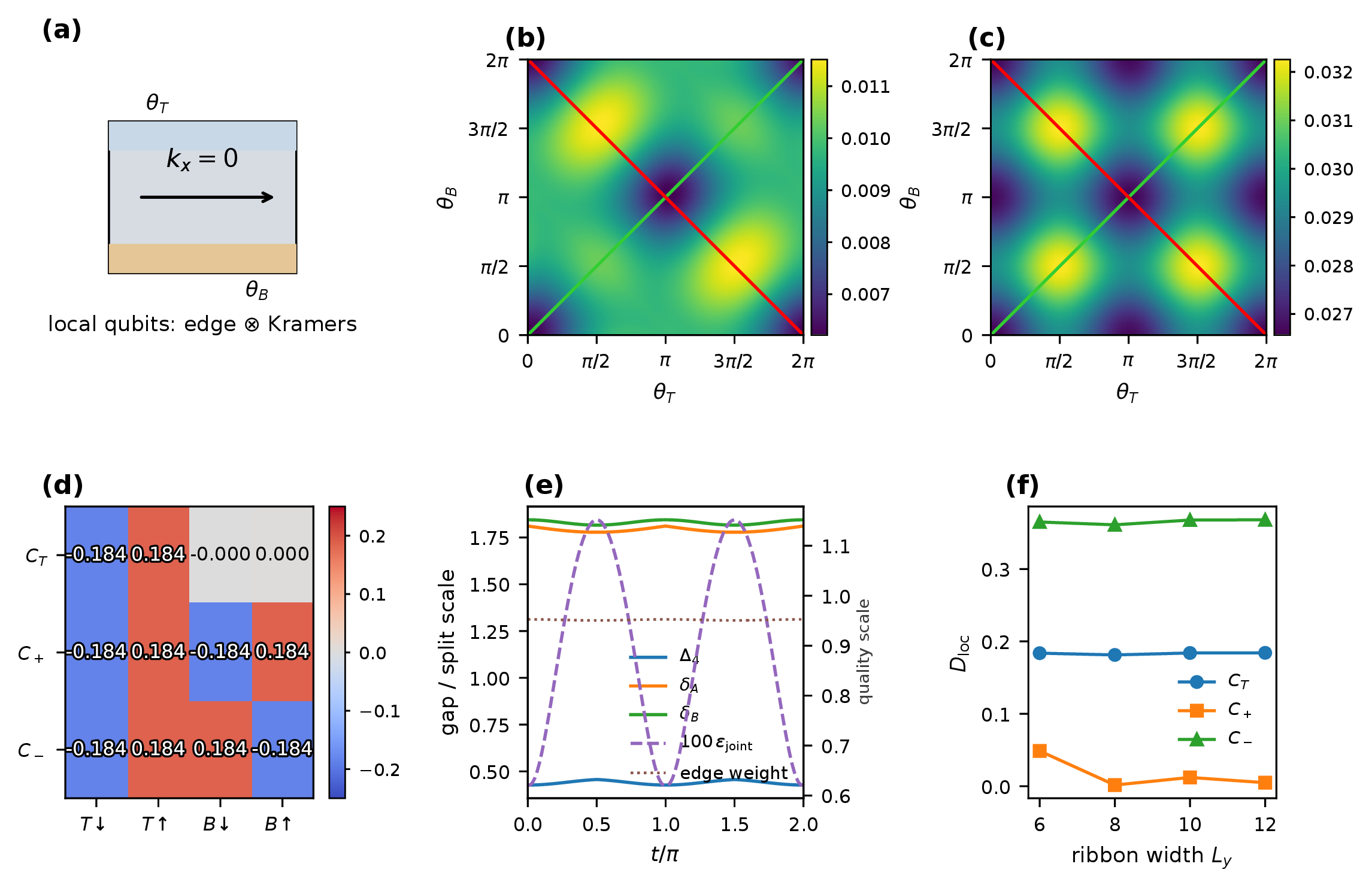
The BHZ model is a four-band lattice description of a two-dimensional quantum spin Hall insulator, with orbital and spin degrees of freedom [1, 16, 17]. In its band-inverted regime, an open ribbon supports counterpropagating helical modes on each boundary. At fixed momentum near the time-reversal-invariant point, the top and bottom edge pairs provide four low-energy states. The in-plane Zeeman terms used below act only on the outer rows. Rotating the top and bottom fields changes the boundary spin texture without changing the bulk hopping, so $({𝜃}_T,{𝜃}_B)$ gives a direct two-parameter control of the edge quartet.

The BHZ ribbon gives the sharpest loop contrast in the present data. On the same helical quartet, co-rotating edge fields remain almost local, while counter-rotation gives an entangling holonomy with nearly the same eigenphase data. This makes the comparison with standard Berry diagnostics especially direct.

We study a ribbon slice at fixed $k_x=\; 0$ with open $y$ direction, independently rotating top and bottom edge Zeeman fields, width $L_y=\; 10$, and parameters $(M,B,A,{\lambda }_R,h_e)\; =\; (1,1,1,0.2,0.6)$ [1, 16, 17]. The control torus is spanned by the edge-field angles $({𝜃}_T,{𝜃}_B)$.

We write ${\tau }_{\mu }$ for the orbital Pauli matrices and ${\sigma }_{\mu }$ for spin, with ${\tau }_0={\sigma }_0=I_2$. With $c_y(k_x)$ the four component row spinor, the Hamiltonian is

$$H_{\mathrm{\text{BHZ}}}(k_x,{𝜃}_T,{𝜃}_B)\; =\underset{y=1}{\overset{L_y}{\sum }}{c}_y^{†}{h}_0(k_x)c_y+\underset{y=1}{\overset{L_y-1}{\sum }}(c_y^{†}{T}_y{c}_{y+1}+\text{h.c.})+c_1^{†}{V}_T({𝜃}_T)c_1+c_{L_y}^{†}{V}_B({𝜃}_B)c_{L_y},$$

(4.1)

with

At $k_x=\; 0$ the $\sin <!--\; FUNCTION\; APPLICATION\; -->k_x$ terms in $h_0$ vanish, but the $y$ hopping still contains the Rashba term proportional to ${\lambda }_R$. The annulus calculation in the next subsection keeps the same Hamiltonian and varies $k_x$.

The compressed observables are ribbon side and a spin-derived label,

$$O_A^{\mathrm{\text{BHZ}}}=\; y,O_B^{\mathrm{\text{BHZ}}}=s_z.$$

(4.6)

Inside the quartet, the first effective qubit is the edge label and the second is the binary label extracted from compressed $s_z$. Although $s_z$ is not conserved once ${\lambda }_R\ne 0$, its compression into the isolated quartet remains well split over the benchmark window and provides a stable helical pseudospin label. In the time-reversal-symmetric limit, this second factor reduces to the Kramers pair at $k_x=\; 0$. With the boundary Zeeman fields present, we refer to it throughout as the extracted helical pseudospin. We denote the corresponding Pauli operators by $Z_{\mathrm{\text{edge}}}$ and $Z_h$, respectively.

The ordered frame is $[T\; \downarrow ,T\; \uparrow ,B\; \downarrow ,B\; \uparrow ]$. Its phases are fixed by requiring positive real amplitudes on the first orbital component of the outer top and bottom rows, respectively:

$${\mathbf{\text{𝐫}}}_{\mathrm{\text{BHZ}}}=(|y\; =\; 1,\mu \; =\; 1,\downarrow ⟩,|y\; =\; 1,\mu \; =\; 1,\uparrow ⟩,|y\; =L_y,\mu \; =\; 1,\downarrow ⟩,|y\; =L_y,\mu \; =\; 1,\uparrow ⟩).$$

(4.7)

Here $\mu \; =\; 1$ denotes the first orbital component of the row spinor. This reference is fixed for the whole control torus and for every BHZ loop.

The quartet remains well isolated over the full edge-angle torus: ${\mathrm{\Delta }}_4^{min}=\; 0.43$, $max\; 𝜖\mathrm{\text{joint}}=\; 0.01$, and the weight in the outer two rows stays above $0.95$. The fixed-slice results are summarized in figure 1. For the symmetry-defined loops

$$C_T:\; ({𝜃}_T,{𝜃}_B)\; =\; (t,0),C_B:\; (0,t),C_{+}:\; (t,t),C_{-}:\; (t,-t),t\; \in \; [0,2\pi ],$$

(4.8)

the response is

$$D\mathrm{\text{loc}}(C_T)\; =\; D\mathrm{\text{loc}}(C_B)\; =\; 0.18,D\mathrm{\text{loc}}(C_{+})\; =\; 0.01,D\mathrm{\text{loc}}(C_{-})\; =\; 0.37.$$

(4.9)

The subscripts in $C_{+}$ and $C_{-}$ label relative edge winding rather than opposite orientations of one loop. In ${\pi }_1(T^2)$, $C_{+}\sim \; (1,1)$ and $C_{-}\sim \; (1,-1)$, whereas the orientation reverse of $C_{+}$ is $(-1,-1)$. Thus $C_{-}$ is not $C_{+}^{-1}$; it is a different primitive cycle that reverses only the bottom-edge field relative to the top-edge field. For any fixed loop $C$, by contrast, reversing its traversal gives $U(C^{-1})\; =\; U{(C)}^{†}$ and leaves $D_{\mathrm{\text{loc}}}$ and $e_p$ unchanged.

On this torus, the same helical quartet supports co-rotation that stays almost local, single-edge cycles with intermediate $D\mathrm{\text{loc}}$, and a counter-rotating entangler. As summarized in table 4, the co-rotating and counter-rotating loops also share the same sorted microscopic eigenphase quadruplet to the reported precision, so the contrast is not explained by eigenphase size alone. At the fitted-generator level this equality is exact because $I\; \otimes Z_h$ and $Z_{\mathrm{\text{edge}}}\otimes Z_h$ share the same eigenvalue multiset $\{\pm \varphi ,\pm \varphi \}$. The microscopic loops inherit this equality up to small higher-order corrections.

The fitted generators separate the three loop classes:

$$K_T\approx \varphi P_T\otimes Z_h,K_{+}\approx \varphi I\; \otimes Z_h,K_{-}\approx \varphi Z_{\mathrm{\text{edge}}}\otimes Z_h,$$

(4.10)

with $P_T=\; (I\; +Z_{\mathrm{\text{edge}}})∕2$, $\varphi \; =\; 0.18$, and a numerically negligible generator-fit residual for $C_{-}$. The counter-rotating loop therefore realizes an Ising-like entangler in the extracted two-qubit frame rather than merely producing a large $D\mathrm{\text{loc}}$ value. Along $C_{-}$ the quartet gap and pointwise quality remain open throughout the cycle, so the signal is not caused by a collapsing local frame.

The connection-level origin separates the common and differential directions on the control torus. Let

$$F({𝜃}_T,{𝜃}_B)\; =(|T,+⟩,|T,-⟩,|B,+⟩,|B,-⟩)$$

(4.11)

be the extracted local frame, ordered as edge label followed by helical pseudospin label. In this frame,

$$A\; =F^{†}dF\; =A_{{𝜃}_T}d{𝜃}_T+A_{{𝜃}_B}d{𝜃}_B,U(C)\; =\mathcal{\text{𝒫}}\exp <!--\; FUNCTION\; APPLICATION\; -->{\oint }_{C}A.$$

(4.12)

The elementary cycles contract the connection with

$$C_T:\; A({Ċ}_T)\; =A_{{𝜃}_T},C_{+}:\; A({Ċ}_{+})\; =A_{{𝜃}_T}+A_{{𝜃}_B},C_{-}:\; A({Ċ}_{-})\; =A_{{𝜃}_T}-A_{{𝜃}_B},$$

(4.13)

up to the common parametrization factor.

At the Hamiltonian level, ${\partial }_{{𝜃}_T}H$ and ${\partial }_{{𝜃}_B}H$ are supported on the top and bottom edges, respectively. After projection to the quartet, the fitted principal-generator channels are

$$K_T\sim \varphi P_T\otimes Z_h,K_B\sim \varphi P_B\otimes Z_h,P_T=\frac{I\; +Z_{\mathrm{\text{edge}}}}{2},P_B=\frac{I\; -Z_{\mathrm{\text{edge}}}}{2}.$$

(4.14)

Both blocks use the same extracted $Z_h$ convention. The opposite propagation directions of the microscopic helical modes are absorbed into the edge-dependent identification of this pseudospin and do not introduce an additional sign between the two projected channels. Consequently,

The first combination lies in the local algebra, whereas the second is an edge-conditioned helical phase transverse to it. The exact calculation retains path ordering: the Wilson loop is computed first and its principal logarithm is then resolved into tensor-product channels.

4.2 Momentum continuation and an experimental signature

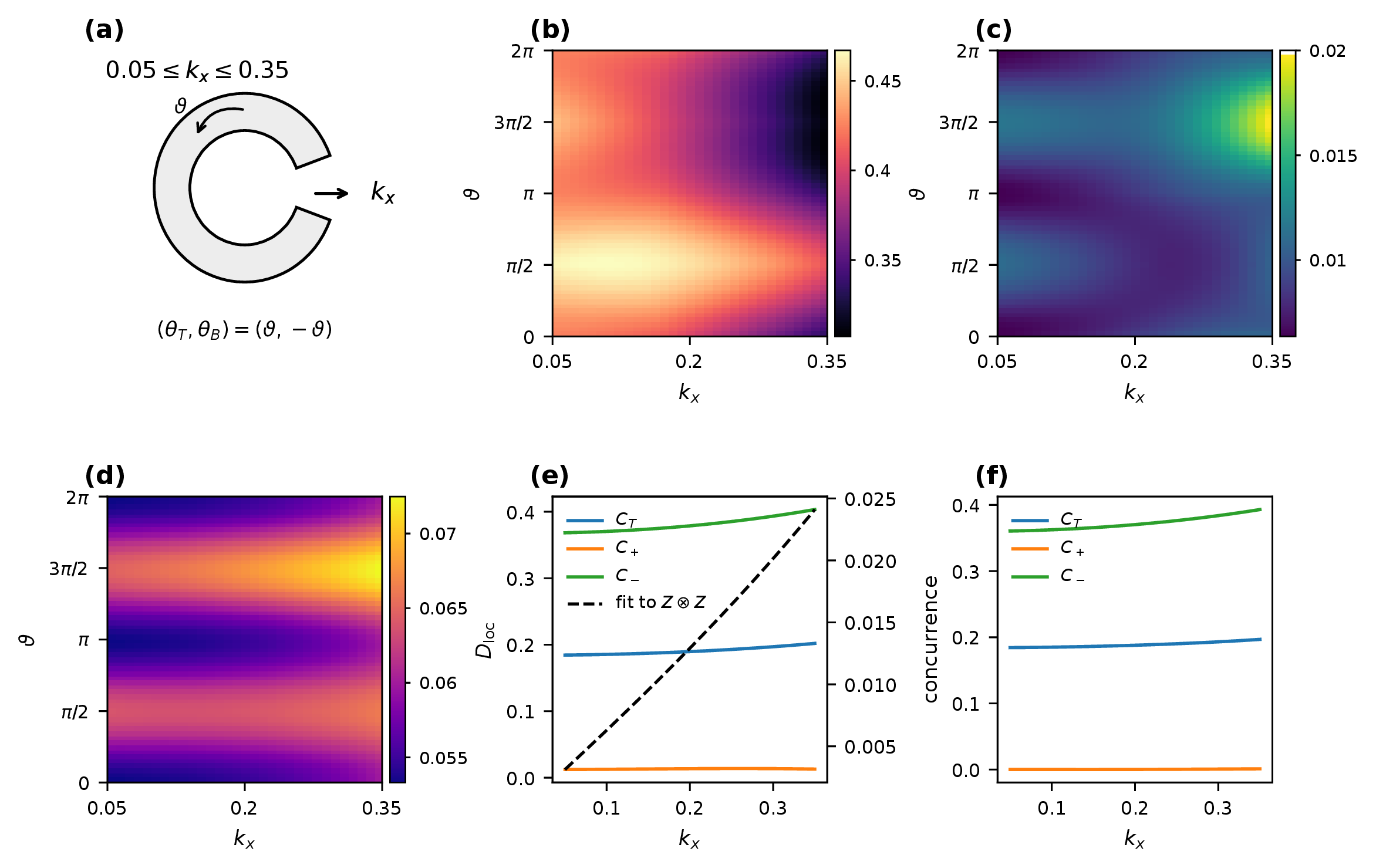
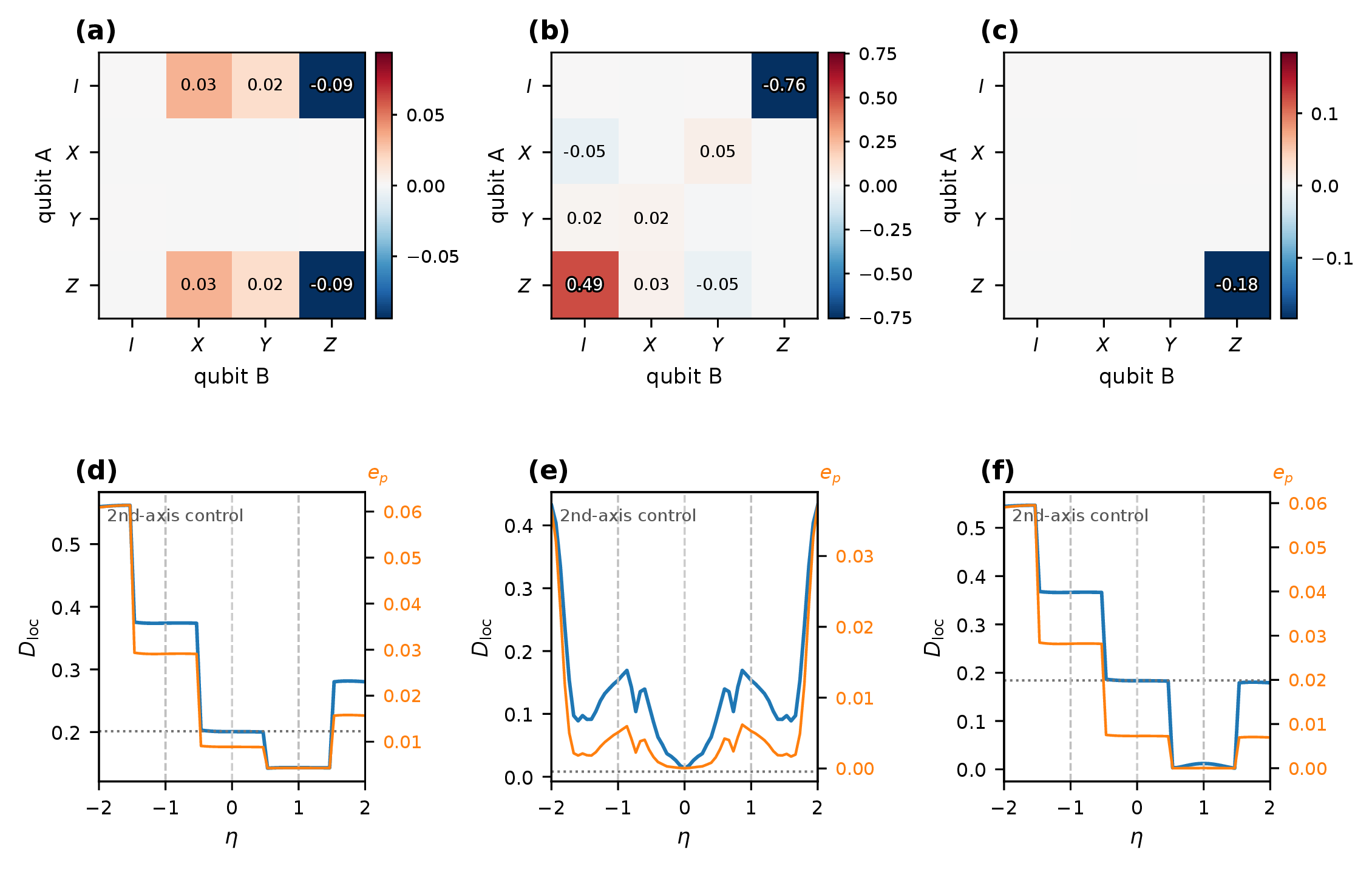
The fixed-$k_x$ ribbon isolates the helical mechanism. We now examine whether the same contrast persists when momentum is allowed to vary. To avoid bulk re-entry we continue the counter-rotating texture to the annulus

$${\mathcal{\text{𝒜}}}_{\mathrm{\text{BHZ}}}=\; \{(k_x,𝜗)\; :k_x\in \; [0.05,0.35],𝜗\; \in \; [0,2\pi )\},({𝜃}_T,{𝜃}_B)\; =\; (𝜗,-𝜗).$$

(4.17)

The model is described by the same Hamiltonian (4.1). Only the control manifold changes. The microscopic operators and the quartet extraction stay the same.

Across this annulus the quartet remains well resolved, with ${\mathrm{\Delta }}_4^{min}=\; 0.31$, $max\; 𝜖\mathrm{\text{joint}}=\; 0.02$, and outer-two-row weight above $0.94$.

The loop dependence survives the momentum continuation. Over the full benchmark window,

$$D\mathrm{\text{loc}}(C_{+})\; \approx \; 0.01,D\mathrm{\text{loc}}(C_{-})\; \approx \; 0.4.$$

(4.18)

The branch containing the representative counter-rotating loop therefore remains entangling while the co-rotating control stays almost local. The holonomy also remains close to the Ising form $e^{-i\varphi Z_{\mathrm{\text{edge}}}\otimes Z_h}$: the best-fit distance stays below approximately $0.02$ across the annulus. The fixed-slice contrast is therefore not confined to a single high-symmetry slice.

The annulus also gives a simple output-state witness. Here $|\; +\; +⟩$ denotes the equal-superposition product state in the extracted local basis. Under $C_{-}$ this state acquires concurrence of approximately $0.4$, while the co-rotating control remains negligible over the same momentum window. The single-edge control remains intermediate, with concurrence of approximately $0.2$. This does not replace direct Wilson-loop or interferometric reconstruction of the full holonomy [14, 15]. It shows instead that failure of local reduction can be converted into a two-qubit entanglement witness and leads naturally to the tomography protocol summarized in section 9. The momentum-resolved annulus results, including the concurrence witness, are summarized in figure 2.

5 SSH chain: controlled-rotation benchmark on an edge quartet

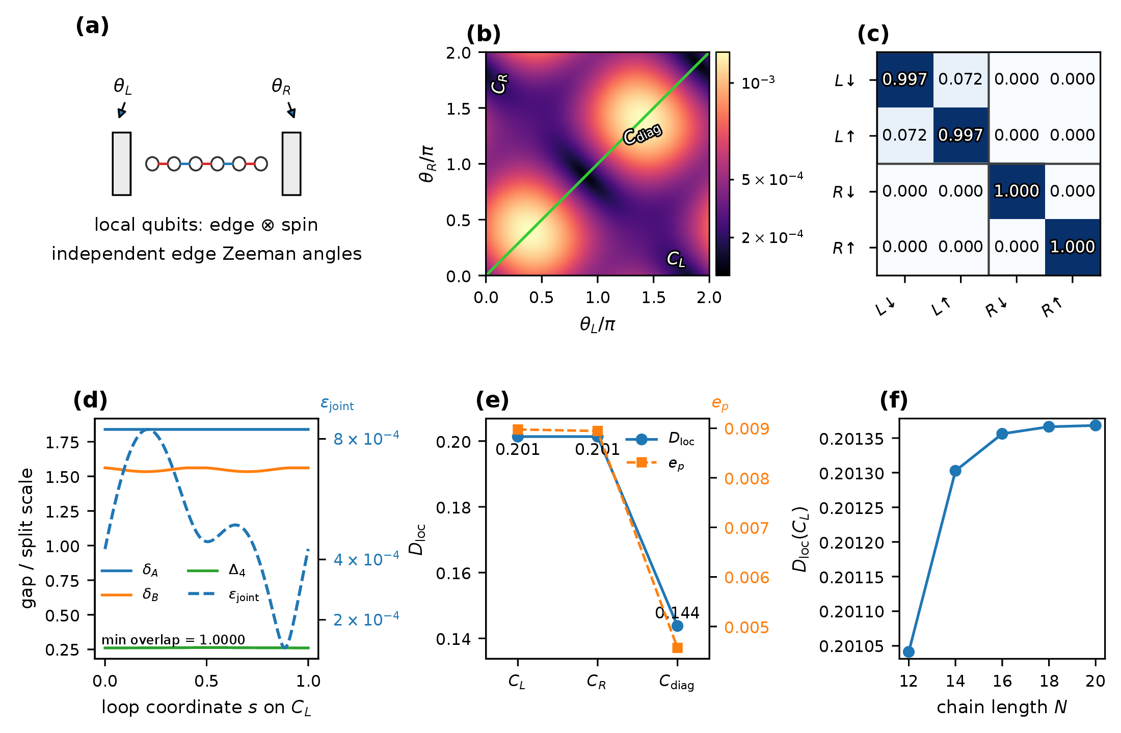
The SSH model is a one-dimensional bipartite chain with alternating intracell and intercell hopping [2, 18]. In the topological dimerization, an open spinless chain has one state localized at each end. Adding spin gives two internal states per end and hence a four-state boundary manifold. In the model below, weak spin-dependent hoppings mix the spin components, while independently rotating fields on the two terminal sites provide the angles $({𝜃}_L,{𝜃}_R)$. The effective binary labels are therefore end position and the spin label resolved inside each end block; the microscopic $A∕B$ sublattice is not used as a logical factor.

The SSH chain provides the numerically most stable benchmark. A single-edge loop acts as a controlled rotation, while the anti-diagonal family gives the larger entangling response. Quartet isolation and split quality are strongest here, so departure from the local subgroup can be followed without collapse of the pointwise local frame.

The model is an open spinful dimerized chain of length $N\; =\; 16$ with independent left and right edge angles,

with

$$T_1=t_{1}I\; +\; i{\lambda }_1{\sigma }_y,T_2=t_{2}I\; +\; i{\lambda }_2{\sigma }_x.$$

(5.3)

We use $(t_1,t_2)\; =\; (0.55,1.0)$, $({\lambda }_1,{\lambda }_2)\; =\; (0.20,0.15)$, and $B\; =\; 0.30$. The intended local structure is $(\text{edge})\; \otimes \; (\text{spin})$, extracted from compressed edge-position and microscopic spin observables.

After the edge and spin lines have been ordered, their phases are fixed by the terminal microscopic orbitals,

$${\mathbf{\text{𝐫}}}_{\mathrm{\text{SSH}}}=(|1A,\downarrow ⟩,|1A,\uparrow ⟩,|NB,\downarrow ⟩,|NB,\uparrow ⟩).$$

(5.4)

The same four references are used for every point and every loop on the SSH control torus.

Across the full torus, ${\mathrm{\Delta }}_4^{min}=\; 0.26$, $max\; 𝜖\mathrm{\text{joint}}=\; 0.001$, and the edge weight stays above $0.60$. The loop dependence remains pronounced. For the symmetry-defined cycles

$$C_L:\; ({𝜃}_L,{𝜃}_R)\; =\; (t,0),C_R:\; (0,t),C_{\mathrm{\text{diag}}}:\; (t,t),C_{\mathrm{\text{anti}}}:\; (t,-t),t\; \in \; [0,2\pi ],$$

(5.5)

we find

$$D\mathrm{\text{loc}}(C_L)\; =\; D\mathrm{\text{loc}}(C_R)\; =\; 0.20,D\mathrm{\text{loc}}(C_{\mathrm{\text{diag}}})\; =\; 0.14.$$

(5.6)

The anti-diagonal loop $C_{\mathrm{\text{anti}}}$ yields the largest response among these symmetry-defined cycles, with $D\mathrm{\text{loc}}(C_{\mathrm{\text{anti}}})\; =\; 0.38$ even though its maximal eigenphase matches that of $C_L$ to the precision shown here. This comparison is revisited in tables 2 and 3. We use $C_L$ as the representative controlled-rotation loop; supplementary scans place it and $C_{\mathrm{\text{anti}}}$ on nearby branches of the same torus. Their canonical coordinates lie on the same one-parameter edge of the Weyl chamber as the corresponding BHZ loops (table 4).

The representative single-edge loop admits a compact effective-generator description. Writing $P_L=\; (I\; +Z_{\mathrm{\text{edge}}})∕2$ for the projector onto the left-edge block, its effective generator is well fit by

$$K_L\approx \varphi P_L\otimes \; (\widehat{n}\cdot \sigma ),\varphi \; =\; 0.20,$$

(5.7)

with $\widehat{n}=\; (0.32,0.16,-0.93)$ and generator residual below $0.001$. The left block rotates while the spectator block remains nearly stationary, giving a controlled rotation on the extracted two-qubit space. Along $C_L$ the quartet gap stays above $0.26$, , and the nearest-neighbor frame overlap stays above $0.99$. The entangling response therefore survives stringent quality checks and varies weakly with system size over the range studied. The SSH benchmark results, including the torus map, representative holonomy, loop comparison, and finite-size dependence, are summarized in figure 3.

6 BBH corner quartet: higher-order reduction failure

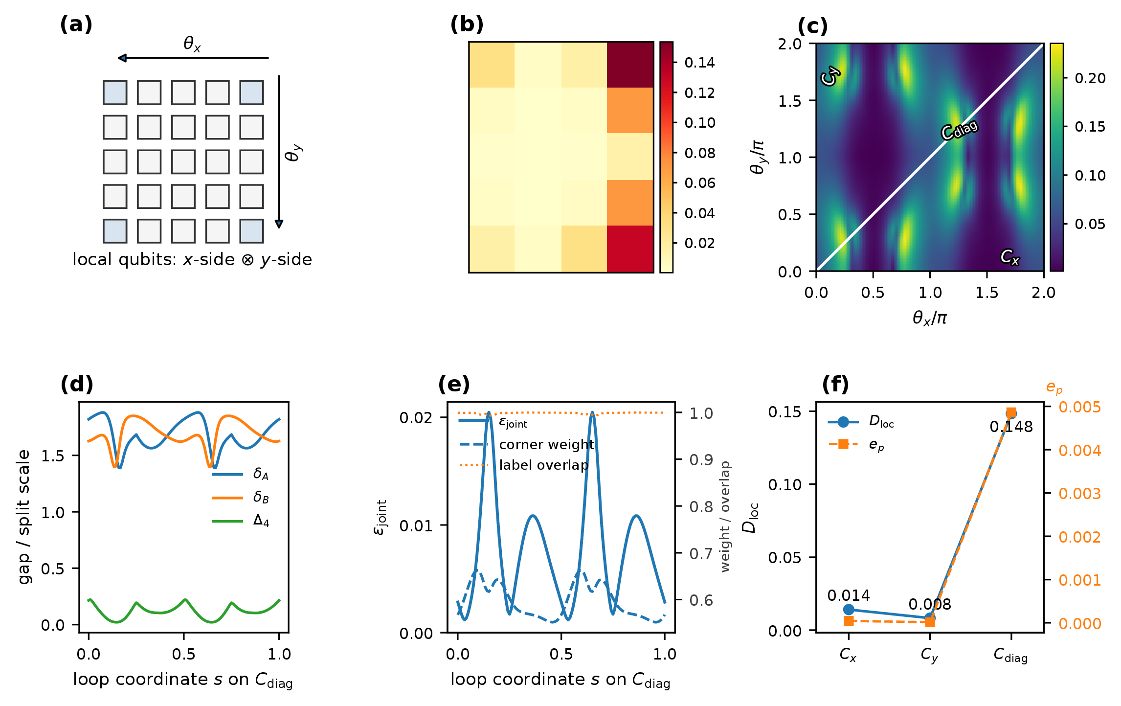
The BBH quadrupole model is a two-dimensional, four-orbital extension of the dimerized-chain construction [3, 19]. In the higher-order topological regime used here, the one-dimensional edges are gapped while localized modes occur at the four corners of an open sample. Those four modes form the quartet. Coarse $x$ position distinguishes left from right, and coarse $y$ position distinguishes bottom from top, producing the $(x\text{-side})\; \otimes \; (y\text{-side})$ structure. The two corner-mass angles rotate local perturbations at the corners while leaving the bulk hopping fixed; they define a control torus, not a momentum-space torus.

BBH extends the analysis beyond first-order edge multiplets. Axis cycles remain almost local, whereas mixed cycles are entangling and explore a more distributed two-qubit gate geometry.

The higher-order extension is the open BBH quadrupole model on a $5\; \times \; 5$ lattice (figure 4(a)) with $({\gamma }_x,{\gamma }_y)\; =\; (0.3,0.3)$, $({\lambda }_x,{\lambda }_y)\; =\; (1,1)$, $\delta \; =\; 0$, and a corner-field torus generated by two angle-dependent corner masses of amplitudes $m_x=m_y=\; 0.6$ [3, 19]. The intended local structure is $(x\text{-side})\; \otimes \; (y\text{-side})$, extracted from coarse position observables compressed into the corner quartet.

With ${\tau }_0={\sigma }_0=I_2$ and $c_{\mathbf{\text{𝐫}}}$ the four component spinor on unit cell $\mathbf{\text{𝐫}}=\; (x,y)$, the Hamiltonian is

$$\begin{array}{cc}\begin{array}{rl}{H}_{\mathrm{\text{BBH}}}({𝜃}_x,{𝜃}_y)& =\underset{\mathbf{\text{𝐫}}}{\sum }{c}_{\mathbf{\text{𝐫}}}^{†}({\gamma }_x{\mathrm{\Gamma }}_4+{\gamma }_y{\mathrm{\Gamma }}_2+\; \delta {\mathrm{\Gamma }}_0)c_{\mathbf{\text{𝐫}}}\\ & +\underset{x=1}{\overset{N_x-1}{\sum }}\sum _{y=1}^{N_y}[c_{x,y}^{†}\frac{{\lambda }_x}{2}({\mathrm{\Gamma }}_4-i{\mathrm{\Gamma }}_3)c_{x+1,y}+\text{h.c.}]\\ & +\underset{x=1}{\overset{N_x}{\sum }}\underset{y=1}{\overset{N_y-1}{\sum }}[c_{x,y}^{†}\frac{{\lambda }_y}{2}({\mathrm{\Gamma }}_2-i{\mathrm{\Gamma }}_1)c_{x,y+1}+\text{h.c.}]\\ & +\underset{\mathbf{\text{𝐫}}\in \mathrm{\text{corners}}}{\sum }{\eta }_{\mathbf{\text{𝐫}}}{c}_{\mathbf{\text{𝐫}}}^{†}[m_x(\cos <!--\; FUNCTION\; APPLICATION\; -->{𝜃}_x{M}_1+\sin <!--\; FUNCTION\; APPLICATION\; -->{𝜃}_x{M}_2)\; +m_y(\cos <!--\; FUNCTION\; APPLICATION\; -->{𝜃}_y{M}_3+\sin <!--\; FUNCTION\; APPLICATION\; -->{𝜃}_y{M}_4)]c_{\mathbf{\text{𝐫}}},\end{array}& \end{array}$$

(6.1)

where

Here $s_x(\mathbf{\text{𝐫}})\; =\; -1$ on the left boundary and $+\; 1$ on the right boundary, while $s_y(\mathbf{\text{𝐫}})\; =\; -1$ on the bottom boundary and $+\; 1$ on the top boundary. The corner sign is ${\eta }_{\mathbf{\text{𝐫}}}=s_x(\mathbf{\text{𝐫}})s_y(\mathbf{\text{𝐫}})$. Both corner fields therefore carry the same corner sign ${\eta }_{\mathbf{\text{𝐫}}}$ and act only on the four corner unit cells. The control torus rotates corner masses and does not modify the bulk hoppings.

The corner lines are ordered as left-bottom, left-top, right-bottom, and right-top. Their phases are completed with

$${\mathbf{\text{𝐫}}}_{\mathrm{\text{BBH}}}=(|1,1;\mu \; =\; 2⟩,|1,N_y;\mu \; =\; 3⟩,|N_x,1;\mu \; =\; 4⟩,|N_x,N_y;\mu \; =\; 1⟩),$$

(6.5)

where $\mu \; =\; 1,\dots ,4$ follows the $\tau \; \otimes \; \sigma$ component ordering used above. These references are held fixed throughout the BBH torus.

The BBH quartet has narrower numerical margins than SSH or BHZ, but the regime of interest remains controlled: on the full torus we find ${\mathrm{\Delta }}_4^{min}=\; 0.02$, $max\; 𝜖\mathrm{\text{joint}}=\; 0.02$, and corner weight above $0.49$. Along the diagonal entangling loop the quality improves further, with ${\mathrm{\Delta }}_4>\; 0.02$, , corner weight above $0.55$, and frame overlap above $0.99$.

For the symmetry-defined cycles

$$C_x:\; ({𝜃}_x,{𝜃}_y)\; =\; (t,0),C_y:\; (0,t),C_{\mathrm{\text{diag}}}:\; (t,t),C_{\mathrm{\text{anti}}}:\; (t,-t),t\; \in \; [0,2\pi ],$$

(6.6)

the loop hierarchy is qualitatively distinct from SSH and BHZ. The axis loops remain nearly local,

$$D\mathrm{\text{loc}}(C_x)\; =\; 0.01,D\mathrm{\text{loc}}(C_y)\; =\; 0.008,$$

(6.7)

whereas both mixed families are entangling,

$$D\mathrm{\text{loc}}(C_{\mathrm{\text{diag}}})\; =\; D\mathrm{\text{loc}}(C_{\mathrm{\text{anti}}})\; =\; 0.15.$$

(6.8)

Axis cycles mainly move one coarse side label at a time and stay near the local subgroup, whereas mixed cycles vary both labels and couple all four corner sectors. The operator-Schmidt spectrum of $C_{\mathrm{\text{diag}}}$ accordingly requires four visible channels, unlike the nearly rank-two SSH and BHZ entanglers, and its fitted generator is spread across several tensor-product channels. Its canonical coordinates contain the first finite second nonlocal coordinate in this set.

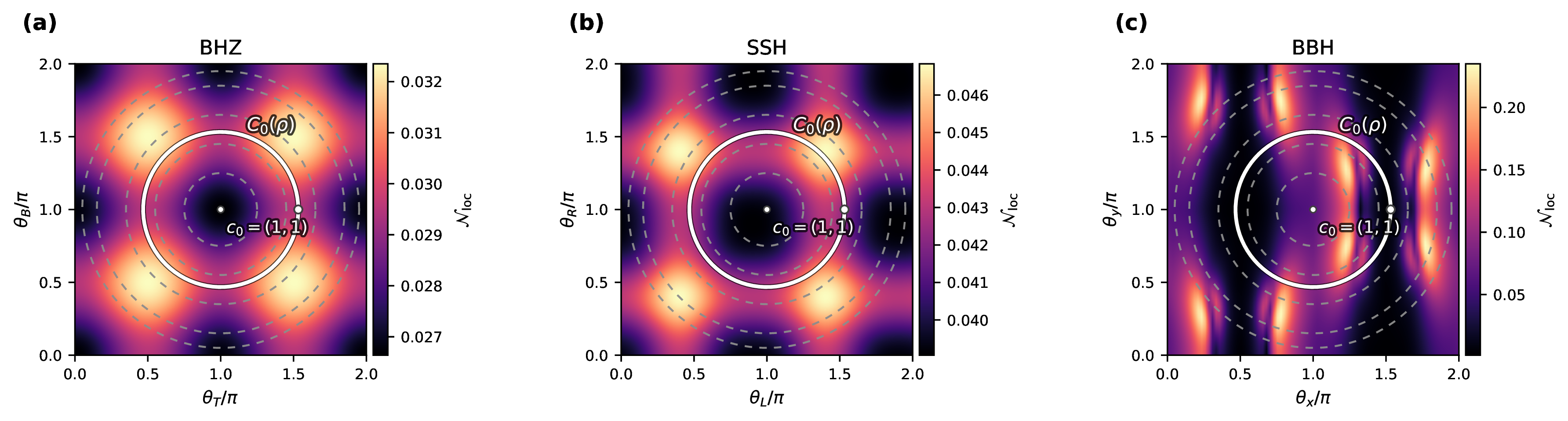
As a null-homotopic control, we also evaluated a center-based family of contractible circles,

$${\mathcal{\text{𝒞}}}_0(\rho )\; :({𝜃}_1,{𝜃}_2)∕\pi \; =c_0+\; \rho (\cos <!--\; FUNCTION\; APPLICATION\; -->t,\sin <!--\; FUNCTION\; APPLICATION\; -->t),c_0=\; (1,1),t\; \in \; [0,2\pi ].$$

(6.9)

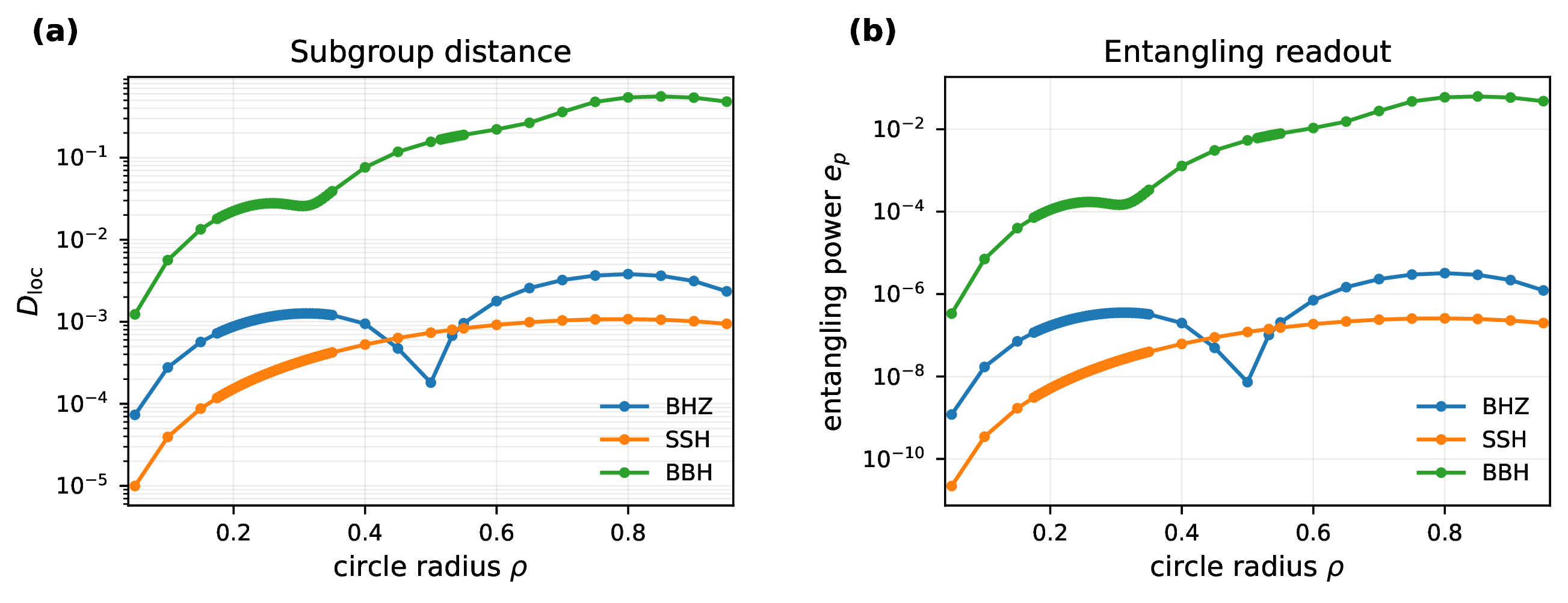
The same center $c_0=\; (1,1)$, radius list, and positive-orientation convention are used in BHZ, SSH, and BBH. Only the physical meaning of $({𝜃}_1,{𝜃}_2)$ changes from model to model. The radius dependence is shown in the Supplementary analyses. In BBH, the contractible-disk scan develops a finite-radius branch with $D_{\mathrm{\text{loc}}}=\mathcal{\text{𝒪}}(10^{-1})$, while the corresponding BHZ and SSH circles remain much smaller on the same geometric family. Since these circles are null-homotopic, this response is not a fundamental-group effect. It comes from the nonlocal component of the quartet Berry curvature over the enclosed disk. Reversing the orientation gives the inverse holonomy, $U_{-}\simeq U_{+}^{†}$, and leaves $D\mathrm{\text{loc}}$ and $ep$ unchanged to numerical precision.

7 Dependence on the phase completion

The references in eqs. (4.7), (5.4), and (6.5) select one tensor-product embedding compatible with the four observable-defined lines. On the representative loop grids, the smallest reference amplitude $|⟨r_{ab}|f_{ab}⟩|$ is $0.76$ for SSH, $0.55$ for BHZ, and $0.53$ for BBH, so none of the selected components vanishes along a named loop.

A general alternative phase completion is $F^{\prime }(\lambda )\; =\; F(\lambda )g(\lambda )$ with a smooth, single-valued diagonal map $g(\lambda )\; \in \mathrm{\text{U}}{(1)}^4$. For a loop based at ${\lambda }_0$, the ordered link product transforms as

$$U^{\prime }(\mathcal{\text{𝒞}})\; =\; g{({\lambda }_0)}^{†}U(\mathcal{\text{𝒞}})g({\lambda }_0).$$

(7.1)

The $\lambda$-dependence of $g$ therefore enters only through its value at the base point. Writing the four phases of $g({\lambda }_0)$ as ${\varphi }_{ab}$ gives

$$g({\lambda }_0)\; =e^{i{\varphi }_{00}}\left[diag\left(1,e^{i({\varphi }_{10}-{\varphi }_{00})}\right)\otimes \; diag\left(1,e^{i({\varphi }_{01}-{\varphi }_{00})}\right)\right]D_{\chi }.$$

(7.2)

The global phase and the tensor product of diagonal one-qubit factors lie in the specified local subgroup, and conjugation by them leaves $D\mathrm{\text{loc}}$ unchanged. A scan over constant $\chi$ thus exhausts the residual diagonal-completion freedom. To determine which conclusions depend on this choice, for each named loop we computed

(7.3)

Since $D_{\chi }$ differs from the identity only on the $|11⟩$line,

$${(D_{\chi }^{†}U{D}_{\chi })}_{jk}=e^{-i\chi {\delta }_{j4}}{U}_{jk}{e}^{i\chi {\delta }_{k4}}.$$

(7.4)

Thus a holonomy with $U_{j4}=U_{4j}=\; 0$ for $j\; =\; 1,2,3$ is exactly completion-independent. This criterion explains the collapsed envelopes of the reported BHZ loops and the SSH single-edge loop to numerical precision.

The criterion above accounts for the completion-independent envelopes of the BHZ loops and SSH $C_L$ ($C_R$) in the numerical data. The SSH anti-diagonal loop also retains a finite lower bound. The BBH mixed-loop case is narrow but nonzero, $[0.148,0.152]$. For BBH $C_{\mathrm{\text{diag}}}$, the off-diagonal entries in the $|11⟩$row and column carry only $5.4\; \times \; 10^{-3}$, or $0.54\%$, of the total Frobenius weight. This small weight explains the narrow phase-completion interval despite the four visible operator-Schmidt channels in table 3: the Schmidt spectrum characterizes the complete operator, whereas the $\chi$ dependence is governed only by these fourth-row and fourth-column entries. The SSH diagonal loop can become local under another completion, while the BBH axis-loop values vary more appreciably. Those secondary values are therefore properties of the physically anchored embedding, not invariants of the four projectors alone. The headline BHZ and SSH loop contrasts survive the residual-phase scan. In BBH, the mixed-loop response remains finite and weakly completion dependent, whereas the quantitative axis-loop classification is tied to the anchored reduction. The phase-completion dependence of all named loops is summarized in table 1.

8 Why standard Berry data do not determine the obstruction

Standard Berry data do not determine the obstruction because they retain phases or spectra of the loop operator but not its position relative to the chosen product subgroup. Chern numbers, determinant phases, and Wilson-loop eigenphases are invariant under the full $\mathrm{\text{U}}(D)$ structure group, whereas locality asks whether $U(C)$ belongs to the embedded subgroup $G_{\mathbf{\text{𝐝}}}$. Isospectral holonomies can therefore have different subsystem-locality classes.

Berry curvature supplies local geometric information, but it must also be read relative to the reduction. Nonzero curvature alone is not the obstruction; the relevant component is the part of the quartet curvature transverse to ${𝔤}_{\mathbf{\text{𝐝}}}$, together with its path-ordered accumulation around the loop.

Formally, let $E\; \to \; X$ be the isolated rank-$D$ bundle and suppose that the compressed observables define a factorization type $\mathbf{\text{𝐝}}=\; (d_1,\dots ,d_r)$, hence an embedded local subgroup $G_{\mathbf{\text{𝐝}}}\subset \mathrm{\text{U}}(D)$ with Lie algebra ${𝔤}_{\mathbf{\text{𝐝}}}$. In an extracted frame $F$, the connection is a one-form

$$A\; =F^{†}dF\; \in {\mathrm{\Omega }}^1(X,𝔲(D)).$$

(8.1)

Using the Hilbert-Schmidt inner product on $𝔲(D)$, choose the orthogonal decomposition

$$𝔲(D)\; ={𝔤}_{\mathbf{\text{𝐝}}}\oplus {𝔪}_{\mathbf{\text{𝐝}}},A\; =A_{\parallel }+A_{\perp },A_{\perp }:=\; (1\; -{\mathrm{\Pi }}_{\mathbf{\text{𝐝}}})A.$$

(8.2)

Under a change of extracted local frame by a $G_{\mathbf{\text{𝐝}}}$-valued gauge transformation, $A_{\perp }$ transforms covariantly by the adjoint action, while $A_{\parallel }$ has the usual inhomogeneous gauge term. Hence the statement that a given tangent direction has a transverse component is local-gauge covariant; it is not a statement about an arbitrary basis of the quartet.

For a path $\gamma$, the holonomy solves

$${\dot{U}}_{\gamma }(t)\; =U_{\gamma }(t)A(\dot{\gamma }(t)),U_{\gamma }(0)\; =\; I.$$

(8.3)

If $A(\dot{\gamma }(t))$ lies in ${𝔤}_{\mathbf{\text{𝐝}}}$ for the entire path in a local gauge, then $U_{\gamma }(t)$ remains in $G_{\mathbf{\text{𝐝}}}$. Conversely, transverse components of $A(\dot{\gamma })$ are the infinitesimal source of subgroup exit, although path ordering can still produce cancellations. For a small contractible loop, the first nontrivial term is controlled by the transverse part of the curvature,

$$U(\partial \mathrm{\Sigma })\; =\; I\; +{\int }_{\mathrm{\Sigma }}{F}_A+\; \cdots ,(1\; -{\mathrm{\Pi }}_{\mathbf{\text{𝐝}}})F_A$$

(8.4)

being the subgroup-relative piece that can generate nonlocal holonomy. Thus the relevant datum is not the Berry curvature alone, but the Berry curvature together with the reduction ${𝔤}_{\mathbf{\text{𝐝}}}\subset \; 𝔲(D)$.

Standard Berry reductions still discard this information. Chern-Weil forms such as $Tr(F_A^k)$, determinant phases, and Wilson-loop eigenphases are invariant under the full structure group $\mathrm{\text{U}}(D)$ and depend only on conjugacy-invariant or trace-level information. The question $U(C)\; \in G_{\mathbf{\text{𝐝}}}$ is not a full-$\mathrm{\text{U}}(D)$ conjugacy question; it depends on the embedding of the product subgroup fixed by the compressed observables. Equivalently, two pairs $(U,G_{\mathbf{\text{𝐝}}})$ can have the same spectrum for $U$ but different answers to the subgroup-membership problem. This is the sense in which the local-reduction obstruction is invisible to Berry data that have forgotten the subsystem reduction.

For a diagonal two-qubit holonomy, the subgroup-relative information can be seen directly. Order the extracted quartet as

$$|T,+⟩,|T,-⟩,|B,+⟩,|B,-⟩,$$

(8.5)

where $T∕B$ is the edge label and $+\; ∕-$ is the helical pseudospin label. In the nearly diagonal regime one may write

$$U(C)\; \simeq \; diag(e^{-i{\alpha }_{T+}},e^{-i{\alpha }_{T-}},e^{-i{\alpha }_{B+}},e^{-i{\alpha }_{B-}}).$$

(8.6)

A genuinely local diagonal phase table can contain a global phase, a phase depending only on the edge label, and a phase depending only on the helical label. If

$$z_T=\; +1,z_B=\; -1,z_{+}=\; +1,z_{-}=\; -1,$$

(8.7)

then such a local table has the form

$${\alpha }_{eh}=\; a\; +\; b{z}_e+\; c{z}_h.$$

(8.8)

The most general real-valued diagonal two-qubit phase table on the four labels, however, also has a fourth Walsh component,

$${\alpha }_{eh}=\; a\; +\; b{z}_e+\; c{z}_h+\; d{z}_e{z}_h.$$

(8.9)

The coefficient $d$ is precisely the edge-helical correlation phase. In the generator it is the coefficient of the interaction term

$$d{Z}_{\mathrm{\text{edge}}}\otimes Z_h,$$

(8.10)

and hence it is the diagonal nonlocal component. Writing the four entries explicitly gives

Taking the mixed difference therefore yields

$$\mathrm{\Delta }={\alpha }_{T+}-{\alpha }_{T-}-{\alpha }_{B+}+{\alpha }_{B-}=\; 4d.$$

(8.13)

Thus $\mathrm{\Delta }$ is the discrete mixed derivative of the phase table on $\{T,B\}\times \{+,-\}$. It annihilates the constant term, the edge-only term, and the helical-only term, and keeps only the product term $z_e{z}_h$. Equivalently, it detects whether the phase table can be written as “row phase plus column phase”. This is the diagonal two-qubit version of the general subgroup-membership question: $\mathrm{\Delta }=\; 0$ is necessary and, within the fixed diagonal branch, sufficient for locality of a diagonal phase gate, whereas $\mathrm{\Delta }\ne 0$ signals an edge-helical interaction phase. For example, the co-rotating BHZ pattern

$$\left(\begin{array}{cc}\hfill +\varphi \hfill & \hfill -\varphi \hfill \\ \hfill +\varphi \hfill & \hfill -\varphi \hfill \end{array}\right)$$

(8.14)

has $\mathrm{\Delta }=\; 0$ and is the local generator $\varphi I\; \otimes Z_h$, while the counter-rotating pattern

$$\left(\begin{array}{cc}\hfill +\varphi \hfill & \hfill -\varphi \hfill \\ \hfill -\varphi \hfill & \hfill +\varphi \hfill \end{array}\right)$$

(8.15)

has $\mathrm{\Delta }=\; 4\varphi$ and is the nonlocal generator $\varphi Z_{\mathrm{\text{edge}}}\otimes Z_h$. Both patterns have the same multiset of phases $\{+\varphi ,+\varphi ,-\varphi ,-\varphi \}$, so a sorted Wilson-loop eigenphase plot sees the same spectrum; the mixed difference sees the placement of those phases relative to the chosen subsystem labels.

The first indication appears at the torus level: using the Fukui-Hatsugai-Suzuki discretization [20], the first Chern number of each quartet bundle is numerically zero, and so are the Chern numbers of the natural rank-two blocks extracted from the local frame. In the present data these quantities are $0$ within numerical resolution. These are not the bulk topological indices of the underlying lattice models; they are Chern numbers of the low-energy quartet bundle over the control torus. For the present question they are silent.

The same is true at the loop level for Abelian phases. For all representative loops in table 2, the determinant phase $\arg <!--\; FUNCTION\; APPLICATION\; -->detU(\mathcal{\text{𝒞}})$ is numerically zero. Nevertheless $D\mathrm{\text{loc}}$ remains finite for the physically important cycles. The local-subgroup obstruction therefore cannot be reduced to a $\mathrm{\text{U}}(1)$ Berry phase.

Wilson-loop eigenphases are more informative than a scalar phase, but they still do not determine whether transport is local or entangling. In SSH, $C_L$ and $C_{\mathrm{\text{anti}}}$ have nearly identical maximal eigenphase, approximately $0.20$, even though their $D\mathrm{\text{loc}}$ values differ by almost a factor of two. In BBH, the almost local loop $C_y$ carries large eigenphases $\pm \; 0.83$ despite $D\mathrm{\text{loc}}(C_y)\; =\; 0.008$. BHZ provides the same comparison in a transparent form. At the fitted low-energy level, the co-rotating and counter-rotating generators $I\; \otimes Z_h$ and $Z_{\mathrm{\text{edge}}}\otimes Z_h$ both produce the eigenphase multiset $\{\pm \varphi ,\pm \varphi \}$; the equality is exact because the two generators differ in subgroup structure, not in eigenvalue content. The microscopic loops inherit that near-degeneracy: to the precision shown in table 4, $C_{+}$ and $C_{-}$ have the same sorted eigenphase quadruplet, even though $D\mathrm{\text{loc}}$ changes from $0.01$ to $0.37$. Canonical Cartan coordinates then separate the loop families: SSH and BHZ lie on the same one-parameter edge of the Weyl chamber, whereas BBH $C_{\mathrm{\text{diag}}}$ develops a finite second nonlocal coordinate. Supplementary operator-Schmidt spectra lead to the same hierarchy without relying only on the fitted-generator picture or on the Frobenius distance.

9 Conclusion and experimental outlook

Across the three models, a pointwise local factorization does not fix the gate class of the loop holonomy. Changing only the loop moves the same quartet between almost local motion, controlled rotations concentrated on one block, and more distributed entanglers. These cases cannot be ordered by a single scalar quantity. Once reduction fails, canonical coordinates place SSH and BHZ on the same one-parameter edge of the two-qubit Weyl chamber, while the BBH mixed cycle develops a finite second nonlocal coordinate.

The quartet language is the smallest explicit form of a dimension-independent statement. For a higher-dimensional boundary multiplet with pointwise labels $(d_1,\dots ,d_r)$, the same analysis replaces $\mathrm{\text{U}}(2)\; \otimes \mathrm{\text{U}}(2)$ by the embedded product subgroup $G_{\mathbf{\text{𝐝}}}$ and asks whether the holonomy reduces to that subgroup. The same issue should arise whenever the connection of the isolated multiplet has curvature or monodromy with a component transverse to ${𝔤}_{\mathbf{\text{𝐝}}}$.

The analysis has two layers. $D\mathrm{\text{loc}}$ asks whether the microscopic holonomy itself lies in the local subgroup. Cartan coordinates, operator-Schmidt spectra, and fitted generators then describe the gate geometry that remains after the holonomy has left that subgroup. Chern numbers, determinant phases, and eigenphase spectra do not answer the subgroup-membership question on their own.

This loop dependence is the microscopic form of the gluing problem studied in ref. [4]. The mathematical formulation is given in the Supplementary analyses. For the present paper, the main point is that a pointwise local factorization can remain well defined while the closed-loop holonomy fails to remain local.

The numerical study is limited to isolated quartets. The higher-dimensional discussion extends the diagnostic framework but is not accompanied by a separate simulation. Quartet selection is guided by symmetry and checked through localization and split diagnostics; the BHZ annulus covers a benchmark momentum window rather than the full Brillouin zone, and BBH has narrower numerical margins than SSH or BHZ. In the trivial-side SSH and BHZ controls and the non-HOTI BBH control, the localization and split-quality conditions fail before a loop-level subgroup interpretation becomes reliable. The conclusions therefore apply to topological boundary quartets within the stated control windows.

Every quoted value of $D\mathrm{\text{loc}}$ is therefore a statement about the phase-complete reduction specified in section 3.1.2 and in the three model sections, not an invariant of the four joint projectors by themselves. Table 1 distinguishes the loop contrasts that remain finite for every residual completion from the secondary controls whose numerical classification depends on that completion.

Possible extensions include larger momentum windows, more realistic helical-edge models on the noninteracting side, higher-dimensional boundary multiplets and many-body edge or ladder quartets obtained from exact diagonalization or tensor-network calculations. The present loop contrast also admits an experimental formulation. Recent experiments already demonstrate non-Abelian adiabatic geometric control and Wilson-loop readout in synthetic settings [14, 21], and related Wilson-loop measurement protocols have been formulated for crystalline systems [15].

Proposed experimental implementation. A practical measurement can be organized in three stages. One first identifies a control window in which the quartet remains isolated by monitoring the quartet gap ${\mathrm{\Delta }}_4$, the split diagnostics, and the relevant localization weight, namely the outer-edge weight in BHZ, the edge weight in SSH, and the corner weight in BBH. Over that window, the compressed observables $(O_A,O_B)$ define the extracted local basis and therefore the product reference states of the effective two-qubit description. One then prepares the product input $|\; +\; +⟩$ in that basis, applies a chosen closed loop, and performs standard two-qubit output-state tomography [22]. Operationally, this uses basis rotations within the quartet together with readout of the compressed observables that define the two labels. Reconstructing ${\rho }_{\mathrm{\text{out}}}(\mathcal{\text{𝒞}})$ gives a direct witness of local-reduction failure through the output concurrence. In BHZ the simplest comparison is $C_{+}$ versus $C_{-}$. In SSH it is $C_L$ versus $C_{\mathrm{\text{anti}}}$. In BBH it is an axis loop versus $C_{\mathrm{\text{diag}}}$.

In this protocol, the observable readouts determine the two binary labels, while calibrated preparation pulses implement the phase completion fixed by the microscopic references in the corresponding model section. The reconstructed operation is therefore tested against the same product reduction used in the numerical calculation.

For a direct determination of the holonomy itself, the witness stage can be upgraded to full quantum process tomography [23] on the extracted two-qubit manifold. Preparing the tensor-product inputs ${\{|0⟩,|1⟩,|+⟩,|\; +\; i⟩\}}^{\otimes 2}$ and performing the same output tomography reconstructs the effective loop channel, from which one can recover the nearest unitary representative, $D\mathrm{\text{loc}}$, and the Cartan coordinates. In a microscopic adiabatic realization, any dynamical contribution can in principle be removed by comparison with a reference sequence or by interferometric calibration of the holonomy [14, 15], so that the reconstructed operator isolates the geometric holonomy rather than the total phase accumulation.

For a higher-dimensional implementation, the reconstruction protocol is unchanged in form. One prepares a tomographically complete set of product inputs in ${\otimes }_{\alpha }{ℂ}^{d_{\alpha }}$, reconstructs the loop channel on the isolated multiplet, and computes $D_{\mathbf{\text{𝐝}}}$ relative to $G_{\mathbf{\text{𝐝}}}$. The witness stage would then use partition-dependent entanglement witnesses or operator-Schmidt diagnostics in place of two-qubit concurrence, while the full process stage would test subgroup membership of the reconstructed holonomy directly.

The three models are not equally demanding experimentally. SSH appears to be the simplest target in the present data because quartet isolation and edge-spin readout margins are strongest there. BHZ requires independent control of top and bottom edge textures and readout calibrated to the extracted helical pseudospin. BBH requires corner-resolved preparation and detection and is therefore more demanding. The extracted two-qubit holonomies can also be implemented on programmable quantum hardware. The accompanying Qiskit implementation realizes representative BHZ, SSH, and BBH extracted-loop circuits, together with output-state tomography and, when needed, full two-qubit process tomography. The same circuit definitions can be run on local Aer simulation or on IBM Quantum backends by changing only the backend specification, with common classical post-processing. Across these implementations, different closed loops on a single boundary quartet produce distinct reduction outcomes.

Acknowledgments

This work was supported by the NSF under Grant No. OSI-2328774 (KI), and by the Israeli Science Foundation Excellence Center, the US-Israel Binational Science Foundation, and the Israel Ministry of Science (YO).

Appendix

A Methods

Quartet projection and pointwise local frame. The construction used in the main text is the rank-four specialization of a general rank-$D$ projection procedure. Given an isolated multiplet with $D\; ={\prod }_{\alpha }{d}_{\alpha }$, one forms $P_D(\lambda )$ from the selected states and compresses a fixed family of physical observables whose joint spectral structure resolves the desired subsystem labels. A viable higher-dimensional local frame requires finite spectral splits for these labels, small incompatibility among the compressed observables, and stable localization of the selected multiplet. The quartet benchmarks below set $D\; =\; 4$ and $\mathbf{\text{𝐝}}=\; (2,2)$, for which two observables resolve and order the four one-dimensional subspaces used in the numerical analysis.

Their phases, and hence the complete tensor-product embedding, are fixed separately by eq. (3.7) and the model-specific references in the main text.

For all three models we work with a smooth Hamiltonian family $H(\lambda )$ and an isolated rank-four projector built from the four low-energy states nearest zero energy,

$$P_4(\lambda )\; =\underset{a=1}{\overset{4}{\sum }}|u_a(\lambda )⟩⟨u_a(\lambda )|.$$

(A.1)

We do not regard the resulting local frame as a unique microscopic tensor product. Instead, we ask whether the loop holonomy stays inside the local subgroup extracted from two physically motivated observables $O_A$ and $O_B$ whose quartet compressions exhibit a well-resolved $2\; +\; 2$ split. The observables themselves need not be binary in the full Hilbert space: in BHZ we use position $y$ and spin $s_z$, and in BBH we use coarse position observables. Binary labels emerge only after compression to the isolated quartet. The pair $(O_A,O_B)$ is fixed once per model from locality and symmetry considerations before any loop-level analysis and is not tuned loop by loop or path by path to maximize $D\mathrm{\text{loc}}$.

The compressed observables are

$${\tilde{O}}_A=P_4{O}_A{P}_4,{\tilde{O}}_B=P_4{O}_B{P}_4,$$

(A.2)

and are sequentially diagonalized to define a pointwise local frame $F(\lambda )\; \in {ℂ}^{N\times 4}$. In SSH these observables resolve edge and spin, in BBH they resolve coarse $x$- and $y$-side labels, and in BHZ they resolve ribbon side and the spin-derived helical pseudospin described in the main text. The construction uses a fixed order: $O_A$ defines the coarse two-block split and $O_B$ resolves each block internally. We do not claim uniqueness of this extraction; rather, the qualitative loop hierarchy is stable across the smooth observable deformations reported in Supplementary figure 8. We also checked the explicit order swap $O_A\leftrightarrow O_B$: in SSH and BHZ the hierarchy among almost local, intermediate, and entangling loops survives with only small numerical shifts, and in BBH the axis-versus-mixed distinction survives as well (Table 6).

The pointwise quality of this factorization is monitored by the quartet gap ${\mathrm{\Delta }}_4$ and by the normalized commutator

$$𝜖\mathrm{\text{joint}}(\lambda )\; =\frac{{\Vert [{\tilde{O}}_A,{\tilde{O}}_B]\Vert }_F}{\mathrm{\text{range}}({\tilde{O}}_A)\mathrm{\text{range}}({\tilde{O}}_B)}.$$

(A.3)

Here ${\Vert X\Vert }_F=\sqrt{Tr(X^{†}X)}$ is the Frobenius norm and $\mathrm{\text{range}}(X)\; ={\lambda }_{max}(X)\; -{\lambda }_{min}(X)$ is evaluated inside the quartet. Small $𝜖\mathrm{\text{joint}}$, combined with a finite quartet gap, indicates that the local two-qubit description is well defined. After diagonalizing ${\tilde{O}}_A$ we use its middle gap to split the quartet into two two-dimensional blocks. Writing the ordered eigenvalues of ${\tilde{O}}_A$ as $a_1\le a_2\le a_3\le a_4$, the corresponding split diagnostic is

$${\delta }_A=a_3-a_2.$$

(A.4)

Inside each $2\; \times \; 2$ block we diagonalize ${\tilde{O}}_B$ and define the block-wise split diagnostic ${\delta }_B$ as the smaller of the two level splittings. These quantities appear in the along-loop quality panels.

Loop holonomies and local-subgroup diagnostics. For neighboring parameter points we define the unitary link

$${\mathcal{\text{𝒰}}}_{\lambda \to {\lambda }^{\prime }}=\mathrm{\text{polar}}(F{(\lambda )}^{†}F({\lambda }^{\prime })),$$

(A.5)

whose ordered product around a closed discretized loop gives the extracted Wilczek-Zee holonomy $U(\mathcal{\text{𝒞}})$. The main loop diagnostic is the reduction-relative distance to the specified local subgroup,

$$D\mathrm{\text{loc}}(\mathcal{\text{𝒞}})\; =\underset{A,B\in \mathrm{\text{U}}(2)}{min}{\Vert U(\mathcal{\text{𝒞}})\; -A\; \otimes B\Vert }_F.$$

(A.6)

For a general factorization type, the numerical objective becomes

$$D_{\mathbf{\text{𝐝}}}(\mathcal{\text{𝒞}})\; =\underset{V_{\alpha }\in \mathrm{\text{U}}(d_{\alpha })}{min}{\Vert U(\mathcal{\text{𝒞}})\; -V_1\otimes \cdots \; \otimes V_r\Vert }_F,$$

(A.7)

with optional minimization over physically allowed permutations of identical factors. In the two-qubit benchmarks this reduces to the displayed $D\mathrm{\text{loc}}$ and, as checked explicitly, allowing the qubit swap does not change the reported classification.

We use entangling power $ep$ [24] only as a secondary descriptor. For the representative named loops quoted in the main text and tables, $ep$ is evaluated exactly from the canonical Cartan coordinates $(c_1,c_2,c_3)$ after removing global phase,

$$ep\; =\frac{1}{18}[3\; -\cos <!--\; FUNCTION\; APPLICATION\; -->(2c_1)\cos <!--\; FUNCTION\; APPLICATION\; -->(2c_2)\; -\cos <!--\; FUNCTION\; APPLICATION\; -->(2c_2)\cos <!--\; FUNCTION\; APPLICATION\; -->(2c_3)\; -\cos <!--\; FUNCTION\; APPLICATION\; -->(2c_3)\cos <!--\; FUNCTION\; APPLICATION\; -->(2c_1)],$$

(A.8)

which is the standard two-qubit linear-entropy entangling power in the Cartan-coordinate convention used in table 4 [24–26]. Independent Monte Carlo checks agree with these exact values within numerical resolution. For all representative loops reported in the main text, the same minimum is obtained even if the minimization is enlarged by allowing an explicit qubit swap; the observed nonlocality is therefore not a qubit-relabeling artifact.

The link-level nonlocal content plotted in some torus and annulus maps is built from the discrete Berry connection on a directed grid step $\delta \lambda$,

$$A(\lambda ;\delta \lambda )\; =\frac{1}{|\delta \lambda |}\log <!--\; FUNCTION\; APPLICATION\; -->[{\mathcal{\text{𝒰}}}_{\lambda \to \lambda +\delta \lambda }],$$

(A.9)

where the principal anti-Hermitian logarithm is used. We compare $A$ with the local Lie algebra ${𝔤}_{\mathbf{\text{𝐝}}}$. For the quartet case $\mathbf{\text{𝐝}}=\; (2,2)$,

$${𝔤}_{\mathbf{\text{𝐝}}}=\; \{X_A\otimes I\; +\; I\; \otimes X_B+\; i\alpha I\; :X_A,X_B\in 𝔰𝔲(2),\alpha \; \in ℝ\},$$

(A.10)

and ${\mathrm{\Pi }}_{\mathbf{\text{𝐝}}}$ denotes the Frobenius-orthogonal projector onto this algebra, implemented by orthogonalizing and normalizing the anti-Hermitian set $\{iI,i{\sigma }_{\mu }\otimes I,iI\; \otimes {\sigma }_{\mu }\}$ with respect to the Frobenius inner product. For general $\mathbf{\text{𝐝}}$, the same notation refers to the one-factor-at-a-time algebra defined in section 3.1 and its Frobenius-orthogonal projector.

The plotted quantity is

$$N\mathrm{\text{loc}}(\lambda )\; ={\Vert A(\lambda ;\delta \lambda )\; -{\mathrm{\Pi }}_{\mathbf{\text{𝐝}}}A(\lambda ;\delta \lambda )\Vert }_F,$$

(A.11)

averaged over the coordinate directions of the underlying torus or annulus grid. The main conclusions do not depend on quantitative use of $N\mathrm{\text{loc}}$, but the maps indicate where nonlocal transport is concentrated in parameter space.

Whenever we quote an effective generator fit, we use the Hermitian principal generator $K$ defined from the spectral logarithm of $U(\mathcal{\text{𝒞}})$. All representative loops satisfy , so the branch is unambiguous on the reported cycles. The quoted generator-fit distance is the Frobenius residual ${\Vert K\; -K_{\mathrm{\text{fit}}}\Vert }_F$, while the complementary operator-Schmidt spectra are obtained by reshaping the holonomy as a two-qubit operator and taking its Schmidt singular values.

Numerical conventions and quartet selection. All torus maps use endpoint-free periodic grids, so the $0$ and $2\pi$ seam is not drawn twice. Loop holonomies are computed on closed grids including the endpoint. The representative named loops are the symmetry-defined axis, diagonal, or counter-diagonal cycles on the corresponding control torus; they are not selected a posteriori to maximize $D\mathrm{\text{loc}}$. The supplementary continuous-$\eta$ scan is included only to indicate how these reference loops extend into nearby branches.

The nearest-neighbor frame-overlap diagnostic used in the along-loop quality panels is

$${\mathrm{\text{ov}}}_{j,j+1}=\underset{a=1,\dots ,4}{min}|⟨f_a({\lambda }_j)|f_a({\lambda }_{j+1})⟩|,$$

(A.12)

after consistent ordering and phase fixing of the extracted basis. In the BBH quality panel the same quantity is labeled “label overlap” to fit the available figure space. The localization weights are model specific: SSH edge weight is the average quartet weight on the two terminal edge orbitals, BHZ outer-two-row weight is the average quartet weight on the first and last two lattice rows, and BBH corner weight is the average quartet weight on the four corner unit cells. The pointwise frame is phase-fixed only after the four observable-defined lines have been extracted.

Within the fixed product reduction, $D\mathrm{\text{loc}}$ is invariant under local basis changes. Nonfactorizing diagonal completions select different reductions and are compared explicitly in section 7.

The quartet-selection rule is intentionally conservative. At each parameter point we choose the four states closest to zero energy, then verify that the resulting quartet has the intended edge or corner localization and that the compressed observables exhibit finite splitting. This is sufficient for the benchmark regimes studied here. For BHZ, the additional restriction to a finite momentum window around $k_x=\; 0$ keeps the helical quartet spectrally separated over both the edge-angle torus and the momentum-angle annulus while avoiding bulk re-entry outside the benchmark window.

B Supplementary analyses

Effective generators and continuous loop families. The effective generators clarify the physical interpretation of the benchmark loops. For SSH, the left-loop generator is concentrated in the $P_L\otimes \; (\widehat{n}\cdot \sigma )$ sector, consistent with a controlled-rotation picture. For BBH, the diagonal-loop generator is distributed across several tensor-product channels rather than being dominated by a single one, which is why the response concentrates on mixed cycles. For BHZ, the representative counter-rotating loop isolates the edge-helical Ising term with a small residual.

A complementary basis-independent view is given by the operator-Schmidt spectra in table 3. The co-rotating BHZ loop is nearly rank one, as expected for an almost local gate. The BHZ counter-rotating loop and the SSH single-edge loop are both close to rank two, consistent with Ising-like and controlled-rotation structures, respectively, while the SSH anti-diagonal loop is a larger rank-two entangler. By contrast, the BBH diagonal loop requires four visible Schmidt channels, reinforcing the picture of a higher-order response spread across several channels. Operator-Schmidt data are not a complete local-equivalence classification of two-qubit gates [25, 26]; here they are used as an additional basis-independent check rather than as a replacement for full canonical invariants.

To place the results in standard two-qubit language, table 4 lists canonical Cartan/Weyl-chamber coordinates after factoring out global phase [25, 26]. Combined with the exact entangling powers reported in table 2, these coordinates reveal a common pattern: $C_T$ and $C_L$ occupy approximately the same one-parameter edge of the chamber, $C_{-}$ and $C_{\mathrm{\text{anti}}}$ move farther along that same edge, and $C_{\mathrm{\text{diag}}}$ is the first case here with a finite second Cartan coordinate. In that standard local-equivalence language, the loop hierarchy remains separated without privileging $D\mathrm{\text{loc}}$, $ep$, or the fitted generators.

The bottom row of figure 5 complements the named cycles by scanning the one-parameter family

$$({𝜃}_1,{𝜃}_2)\; =\; (t,\eta t),\eta \; \in \; [-2,2].$$

(B.1)

For integer $\eta$ this is a closed straight-slope loop on the torus. For non-integer $\eta$, however, the path is closed only after appending a short return segment. The continuous scan is therefore an auxiliary visualization of connected branches in slope space, not a length-normalized optimization over all closed loops at fixed slope. The main-text claims are tied to the symmetry-defined representative loops, while the auxiliary scan shows how those representative loops sit inside nearby branches.

For SSH, the anti-diagonal branch around $\eta \; \approx \; -1$ attains larger values than the diagonal branch near $\eta \; \approx \; +1$, while the axis controls remain between them. For BBH, the axis sector stays near local while mixed cycles carry the larger response over a broad region of slope space. For BHZ, the separation is strongest: the branch containing the representative counter-rotating loop near $\eta \; =\; -1$ remains entangling, the co-rotating branch near $\eta \; =\; +1$ stays almost local, and the single-edge control remains between those two branches. Values outside the exact symmetry points should therefore be read as branch diagnostics rather than as a ranking of closed loops by a universal cost function.

Contractible center-based controls. To separate loop homotopy from Berry-curvature effects without selecting a single contractible loop by hand, we computed a center-based radius scan in each control torus. In normalized coordinates the family is

$${\mathcal{\text{𝒞}}}_0(\rho )\; :({𝜃}_1,{𝜃}_2)∕\pi \; =\; (1,1)\; +\; \rho (\cos <!--\; FUNCTION\; APPLICATION\; -->t,\sin <!--\; FUNCTION\; APPLICATION\; -->t),\rho \; =\; 0.05,0.10,\dots ,0.95.$$

(B.2)

All three models use the same center, the same radius scan and the same positive-orientation convention. Figure 6 overlays this common family on ${\mathcal{\text{𝒩}}}_{\mathrm{\text{loc}}}$ maps with periodic edge filling, and figure 7 and table 5 give the radius dependence and an orientation check at the representative radius $\rho \; =\; 0.53$. The result is not isolated to a single tuned circle: BBH develops an extended finite-radius branch with $D_{\mathrm{\text{loc}}}=\mathcal{\text{𝒪}}(10^{-1})$ and continues to larger values at larger radii, while BHZ and SSH remain small on the same geometric family.

Because these circles are null-homotopic, their response probes the Berry curvature enclosed by the disk rather than a nontrivial element of ${\pi }_1(T^2)$. In the extracted frame, the relevant infinitesimal component is $(1\; -{\mathrm{\Pi }}_{\mathbf{\text{𝐝}}})F_A$; after path ordering, its integrated effect can take the holonomy outside $\mathrm{\text{U}}(2)\; \otimes \mathrm{\text{U}}(2)$.

For a fixed circle, reversing the orientation replaces the holonomy by its inverse, so $U_{-}\simeq U_{+}^{†}$ and the subgroup distance is unchanged. This differs from the BHZ comparison of $C_{+}\sim \; (1,1)$ with $C_{-}\sim \; (1,-1)$, which are distinct primitive cycles rather than opposite traversals of one path. The contractible controls therefore isolate curvature-driven path dependence without invoking topological winding.

Relation to ref. [4]. This relation is dimension-independent. Ref. [4] treats a general factorization type $\mathbf{\text{𝐝}}=\; (d_1,\dots ,d_r)$. The present $G_{(2,2)}$ case is the smallest member of that family that can exhibit a nonlocal product-subgroup obstruction. Higher-dimensional boundary multiplets would replace the stabilizer $G_{(2,2)}$ by $G_{\mathbf{\text{𝐝}}}$ without changing the reduction logic.

Ref. [4] asks a global existence question for subsystem structures on twisted projective families. Its mathematical core is a reduction theorem. For a chosen factorization type $d\; =\; (d_1,\dots ,d_r)$, a global product-state locus exists precisely when the underlying ${\mathrm{\text{PGL}}}_n$-torsor reduces to the corresponding stabilizer $G_d$. The resulting subsystem structures are parametrized by $P∕G_d$ and can be realized as a relative Hilbert-scheme locus. Here we fix a spectrally isolated rank-four boundary quartet and one observable pair $(O_A,O_B)$ for each model, and ask a loopwise question instead. Which microscopic holonomies stay inside the extracted local subgroup, and which leave it? In that sense, the condensed-matter result is a loopwise counterpart of ref. [4], not a reformulation of its global existence theorem.

This obstruction should be distinguished from a Brauer-class obstruction. The present quartet is realized inside a globally defined microscopic Hilbert space. After projection to the isolated four-state bundle, the associated algebra of endomorphisms is of the form $End(E)$ and is therefore Brauer-trivial. The relevant obstruction is the finer subsystem-reduction obstruction identified in ref. [4]. Even when the Brauer class is zero, a projective torsor or its gluing functions may fail to reduce to the stabilizer $G_{(2,2)}$. In the present unitary setting, this becomes the loopwise subgroup-membership test $U(\mathcal{\text{𝒞}})\; \in \mathrm{\text{U}}(2)\; \otimes \mathrm{\text{U}}(2)$. If the test fails, the loop glues the extracted product structure by an entangling element, but it does not define a new Brauer class.

For the present rank-four setting with factorization type $(2,2)$, the stabilizer in ref. [4] is the projective counterpart of local two-qubit transformations. Transition functions of an abstract projective torsor are replaced here by holonomies of an isolated boundary quartet. Noncontractible cycles probe global gluing data of the quartet connection. Contractible circles probe the same reduction question infinitesimally through the nonlocal component of the non-Abelian Berry curvature. In both cases the point is not whether the loop is topologically nontrivial. The point is whether the associated gluing operator preserves the extracted product structure.

Observable robustness and controls.

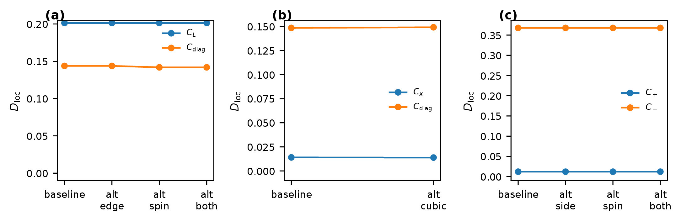
Because the construction starts from two compressed observables, robustness under observable choice must be checked. We therefore varied the coarse edge and spin-like observables in all three models. The results are summarized in figure 8. In SSH the left loop remains at $0.20$ while the diagonal loop stays near $0.14$ under rotated spin-like observables. In BBH the axis loop stays at $0.01$ and the diagonal loop near $0.15$ under cubic coarse position observables. In BHZ the co-rotating and counter-rotating distances are unchanged within plotting resolution under both side-smoothing and rotated spin-like observables. The loop-dependent pattern is therefore not an artifact of any particular observable choice. Because the extraction uses a fixed order, we also exchanged the roles of $O_A$ and $O_B$ on the representative loops. Table 6 shows that this changes the numbers only slightly: SSH and BHZ keep the hierarchy among almost local, intermediate, and entangling loops, and BBH keeps the axis-versus-mixed separation.

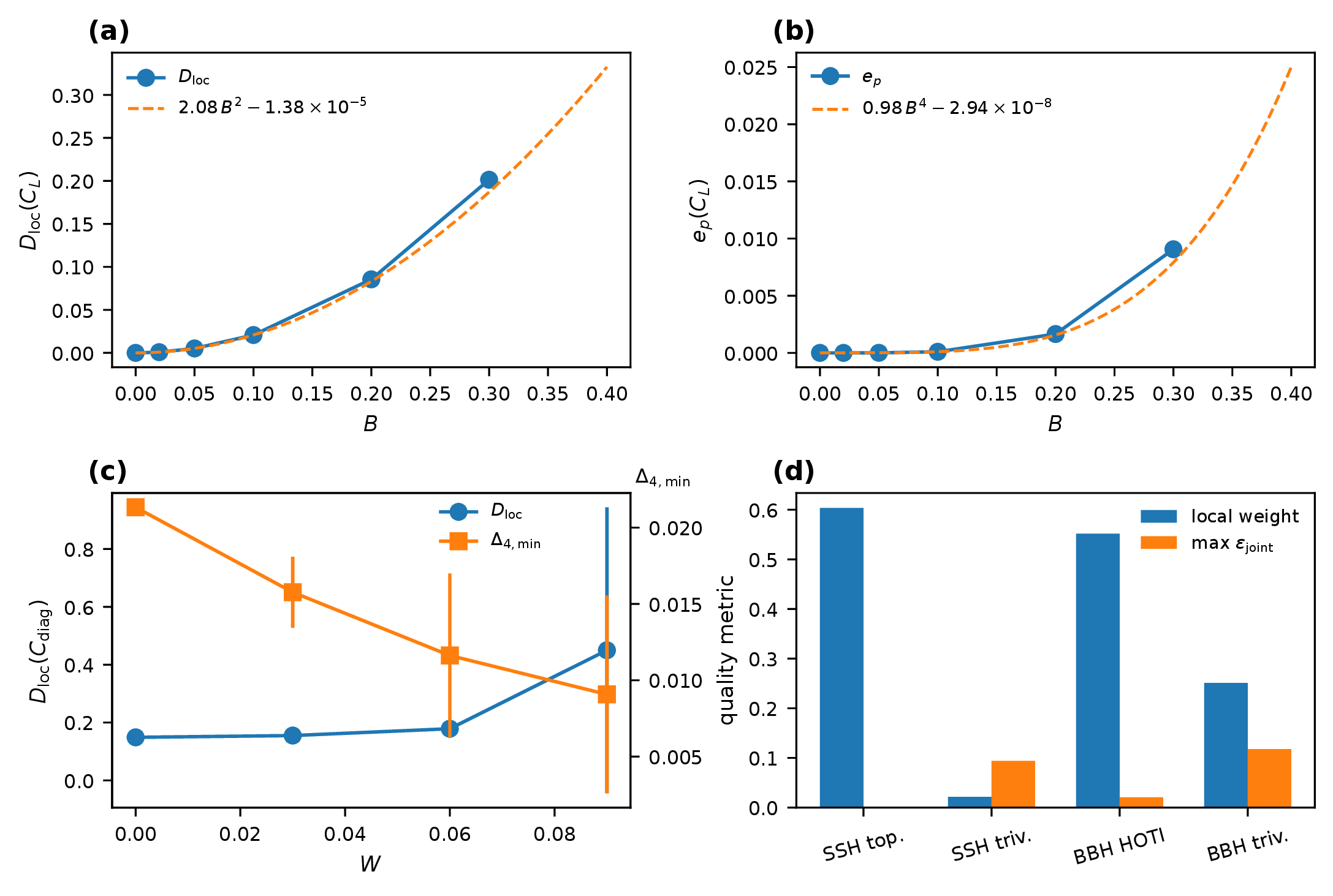
The small-$B$ SSH control shows a perturbative onset with the microscopic driving. For weak $B$,

$$D\mathrm{\text{loc}}(C_L)\; \propto B^2,e\; p(C_L)\; \propto B^4.$$

(B.3)

This indicates a perturbative origin for the local-subgroup obstruction rather than a threshold artifact. The additional weak-driving, disorder, and trivial-phase controls are summarized in figure 9.

The BBH disorder protocol exhibits a controlled weak-disorder regime rather than broad robustness. In that regime the average diagonal-loop distance remains near $0.16$, while at larger disorder the variance grows and the quartet gap is reduced. The appropriate interpretation is therefore stability only before quartet degradation sets in.

Finally, trivial-phase controls show that a topological low-energy multiplet is a necessary prerequisite for the present benchmark. On the trivial SSH side the edge weight collapses to approximately $0.02$, $max\; 𝜖\mathrm{\text{joint}}$ rises to approximately $0.09$, and the minimal gap drops to approximately $0.03$. On the non-HOTI BBH side the corner weight falls to approximately $0.25$ and $max\; 𝜖\mathrm{\text{joint}}$ rises to approximately $0.12$. A matching BHZ trivial control at $M\; =\; 5$ makes the same point in BHZ itself: at fixed $k_x=\; 0$, the minimal quartet gap drops to $0.16$, the outer-two-row weight to $0.19$, and $max\; 𝜖\mathrm{\text{joint}}$ rises to $0.91$. In all three cases the four-state truncation ceases to be a reliable edge or corner benchmark before any loop-level interpretation becomes reliable.

References

[1]

B.A. Bernevig, T.L. Hughes and S.-C. Zhang, Quantum Spin Hall Effect and Topological Phase Transition in HgTe Quantum Wells, Science 314 (2006) 1757 [INSPIRE].

[2]

W.P. Su, J.R. Schrieffer and A.J. Heeger, Solitons in polyacetylene, Phys. Rev. Lett. 42 (1979) 1698 [INSPIRE].

[3]

W.A. Benalcazar, B.A. Bernevig and T.L. Hughes, Quantized electric multipole insulators, Science 357 (2017) 61 [INSPIRE].

[4]

K. Ikeda, Quantum Entanglement Geometry on Severi-Brauer Schemes: Subsystem Reductions of Azumaya Algebras, arXiv:2601.13764 [INSPIRE].

[5]

M.V. Berry, Quantal phase factors accompanying adiabatic changes, Proc. Roy. Soc. Lond. A 392 (1984) 45 [INSPIRE].

[6]

F. Wilczek and A. Zee, Appearance of Gauge Structure in Simple Dynamical Systems, Phys. Rev. Lett. 52 (1984) 2111 [INSPIRE].

[7]

P. Zanardi and M. Rasetti, Holonomic quantum computation, Phys. Lett. A 264 (1999) 94 [quant-ph/9904011] [INSPIRE].

[8]

E. Sjöqvist et al., Non-adiabatic holonomic quantum computation, New J. Phys. 14 (2012) 103035 [arXiv:1107.5127] [INSPIRE].

[9]

R. Yu, X.L. Qi, A. Bernevig, Z. Fang and X. Dai, Equivalent expression of ${𝕫}_2$ topological invariant for band insulators using the non-abelian berry connection, Phys. Rev. B 84 (2011) 075119.

[10]

A.A. Soluyanov and D. Vanderbilt, Computing topological invariants without inversion symmetry, Phys. Rev. B 83 (2011) 235401.

[11]

A. Alexandradinata, X. Dai and B.A. Bernevig, Wilson-Loop Characterization of Inversion-Symmetric Topological Insulators, Phys. Rev. B 89 (2014) 155114 [arXiv:1208.4234] [INSPIRE].

[12]

D. Gresch et al., Z2Pack: Numerical Implementation of Hybrid Wannier Centers for Identifying Topological Materials, Phys. Rev. B 95 (2017) 075146 [arXiv:1610.08983] [INSPIRE].

[13]

B. Bradlyn and M. Iraola, Lecture notes on Berry phases and topology, SciPost Phys. Lect. Notes 51 (2022) 1 [arXiv:2111.08751] [INSPIRE].

[14]

S. Sugawa et al., Wilson loop and Wilczek-Zee phase from a non-Abelian gauge field, npj Quantum Inf. 7 (2021) 144 [arXiv:1910.13991] [INSPIRE].

[15]

A.C. Tyner et al., In-plane Wilson loop for measurement of quantized non-Abelian Berry flux, Phys. Rev. B 109 (2024) 195149 [INSPIRE].

[16]

M.Z. Hasan and C.L. Kane, Colloquium: Topological insulators, Rev. Mod. Phys. 82 (2010) 3045 [arXiv:1002.3895] [INSPIRE].

[17]

X.L. Qi and S.C. Zhang, Topological insulators and superconductors, Rev. Mod. Phys. 83 (2011) 1057 [arXiv:1008.2026] [INSPIRE].

[18]

M.J. Rice and E.J. Mele, Elementary Excitations of a Linearly Conjugated Diatomic Polymer, Phys. Rev. Lett. 49 (1982) 1455.

[19]

F. Schindler et al., Higher-order topological insulators, Sci. Adv. 4 (2018) eaat0346 [arXiv:1708.03636] [INSPIRE].

[20]

T. Fukui, Y. Hatsugai and H. Suzuki, Chern Numbers in Discretized Brillouin Zone: Efficient Method of Computing (Spin) Hall Conductances, J. Phys. Soc. Jap. 74 (2005) 1674 [cond-mat/0503172] [INSPIRE].

[21]

F. Leroux et al., Non-Abelian adiabatic geometric transformations in a cold strontium gas, Nature Commun. 9 (2018) 3580 [arXiv:1802.08418] [INSPIRE].

[22]

D.F.V. James, P.G. Kwiat, W.J. Munro and A.G. White, Measurement of qubits, Phys. Rev. A 64 (2001) 052312 [quant-ph/0103121] [INSPIRE].

[23]

I.L. Chuang and M.A. Nielsen, Prescription for experimental determination of the dynamics of a quantum black box, J. Mod. Opt. 44 (1997) 2455 [quant-ph/9610001] [INSPIRE].

[24]

P. Zanardi, C. Zalka and L. Faoro, Entangling power of quantum evolutions, Phys. Rev. A 62 (2000) 030301(R) [quant-ph/0005031] [INSPIRE].

[25]

Y. Makhlin, Nonlocal Properties of Two-Qubit Gates and Mixed States, and the Optimization of Quantum Computations, Quant. Inf. Proc. 1 (2002) 243 [quant-ph/0002045] [INSPIRE].

[26]

J. Zhang, J. Vala, S. Sastry and K.B. Whaley, Geometric theory of nonlocal two-qubit operations, Phys. Rev. A 67 (2003) 042313 [quant-ph/0209120] [INSPIRE].