

1 Introduction
In the past decade, quantum circuits have emerged as an extremely powerful tool in the study of both integrable and chaotic quantum many-body dynamics [1–17]. In particular, in the context of out-of-equilibrium dynamics of chaotic quantum many-body systems, random unitary circuits (RUCs) provide a simple, tractable model that, via a discretization of the time evolution, allows one to obtain exact results on the spread of correlations and entanglement growth [18–25]. Although RUCs capture the typical behaviour of chaotic systems, circuits built from different classes of random gates can display richer dynamics. One such model that has gained considerable interest lately is the random quantum automaton circuit (QAC) [26, 27]. The QAC dynamics features very similar physics to RUCs when acting on a generic initial state, however, when restricted to appropriately chosen computational basis the dynamics is completely classical and there is no superposition creation. Generally, the QA gates consist of a random permutation of the computational basis, followed by a random phase transformation. The QAC dynamics is closely related to that of random permutation circuits [28], although the presence of random phases make it more analytically tractable. Similar sets of quantum operations which act classically on the computational basis states were studied in integrable condensed matter models [29, 30].
Quantum automaton circuits, together with random permutation circuits for local dimension larger than , display features of quantum chaotic systems [31], although they generally produce sparse wavefunctions when acting on highly localized states in the Hilbert space. One of the most striking differences between RUCs and QACs is that the latter preserve the participation entropy of the initial state in the computational basis. The participation entropy quantifies the extent to which the state is localized (or spread) in the Hilbert space, and the measure of this localization cannot change in time under QAC evolution. This has profound consequences on the entanglement growth in quantum automaton circuits, as well as in random permutation circuits, which were explored in refs. [28, 32]: most notably, the participation entropy of the initial state places an upper bound on the entanglement entropy that can be reached in the stationary state.
The remarkable features of QACs can be better appreciated in the context of quantum resource theories (QRTs) [33]. In a QRT, one indirectly studies a quantity of interest, called a resource, by defining the free states for that resource, which do not display it, and the free operations, which cannot increase it. Resourceful states, on the other hand, can display a large amount of the resource. A classic example of a QRT is that of entanglement [34–37], where free states (i.e. zero entanglement states) are product states, and free operations are local operations and classical communications (LOCC). Any permutation of the states in a given basis followed by a phase transformation is a free operation for the QRT of coherence [33, 38–41], in which free states correspond to density matrices with no off-diagonal elements in a specified basis. Indeed, an incoherent initial state will remain so under evolution with a quantum automaton circuit, since no coherent superposition of basis states can develop if the participation entropy is preserved during the evolution. The QRT of coherence has recently been explored in the context of ergodic quantum many-body dynamics and random quantum circuits [42–49].
In this work, we focus on entanglement asymmetry, introduced two decades ago as a well-behaved quantifier of the quantum resource of asymmetry, or frameness [50–52]. In this QRT, free states are those which commute with a certain symmetry (in our case, global symmetry), and free operations can only produce symmetric states. Resourceful states, the ones which do not display the symmetry, can be employed in experiments and communication protocols involving exchanges between parties that do not have a shared reference frame. More recently, entanglement asymmetry was adopted in the context of quantum many-body systems as a probe of explicit or spontaneous symmetry breaking in a quantum many-body state [53, 54]. Since the first works on entanglement asymmetry in quantum many-body systems, the interest in this quantity has consistently grown -particularly in out-of-equilibrium settings, where symmetry restoration can display a quantum Mpemba effect [55–76]. Many significant works on entanglement asymmetry have appeared in the context of random circuits and typical quantum many-body states [77–82], conformal and quantum field theory [83–93], in relation with generalized symmetries [94–96] and with other QRTs [97]. Moreover, the out-of-equilibrium behaviour of entanglement asymmetry has been recently probed in quantum simulations [82, 98, 99].
We study two ensembles associated to quantum automatons. First, we focus on the setting where some initial pure state is transformed via a global all-to-all gate consisting of a random permutation of the computational basis states followed by a global phase transformation. We call this the quantum automaton ensemble (QAE). Later, we build random circuits consisting of two-body QA gates, where each gate can act on any two qubits randomly, independently of their distance. These 2-local circuits have attracted considerable attention lately [32, 80, 100], for two reasons. On the one hand, two-local circuits are known to be fast scramblers [100], meaning that they equilibriate on a timescale that is logarithmic in the system size. On the other hand, due to the relaxation of the locality constraint and the site-permutation invariance of the evolution operator, some quantities such as the Rényi-2 entanglement entropy admit a Markovian evolution that can be captured through a set of ordinary linear differential equations. Remarkably, the number of linear ODEs is polynomial in the system size.
In both of these settings, we focus on entanglement asymmetry averaged over the respective ensembles. In spin chains, it is naturally associated to a particle number symmetry or to the total magnetization. Remarkably, the stationary value of the entanglement asymmetry of a subsystem in a RUC strongly depends on the size of the subsystem. In ref. [80], it was shown that an initial symmetric state will, at large times, remain symmetric locally: the asymmetry of any subsystem smaller than half the size of the total system vanishes exponentially fast after a relaxation time. Conversely, the asymmetry of a subsystem larger than half the system size at large times reaches the typical value of half the maximum asymmetry (the origin of this typicality was explained in ref. [101]). The same picture holds for the average asymmetry of a subsystem in a Haar random ensemble [78]. As we will show in this work, in a quantum automaton ensemble and in quantum automaton circuits this picture changes drastically due to the conservation of the participation entropy (or total coherence) of the initial state. While on scales we always observe symmetrization, this scale depends on the initial state. Indeed, our first main result is that the competition between uniform exploration of charge sectors and preservation of the participation entropy leads to a shift of the threshold scale until which symmetrization occurs. In particular, this shift depends on the participation entropy of the initial state. This dependence is reminiscent of how the Page curve [102, 103] for the average purity in QACs, as well as in random permutation circuits, depends on the initial state [32]. However, the peculiar phenomenology of entanglement asymmetry in QACs cannot be entirely inferred from the entanglement Page curves. Rather, as we show, the symmetrization scale is closely related to growth of the average subsystem coherence. Indeed, our second main result is that the subsystem size at which late-time symmetrization ceases to occur is the same at which one starts to observe an extensive relative entropy of coherence in the subsystem. Figure 1 contains a sketch of our main results.
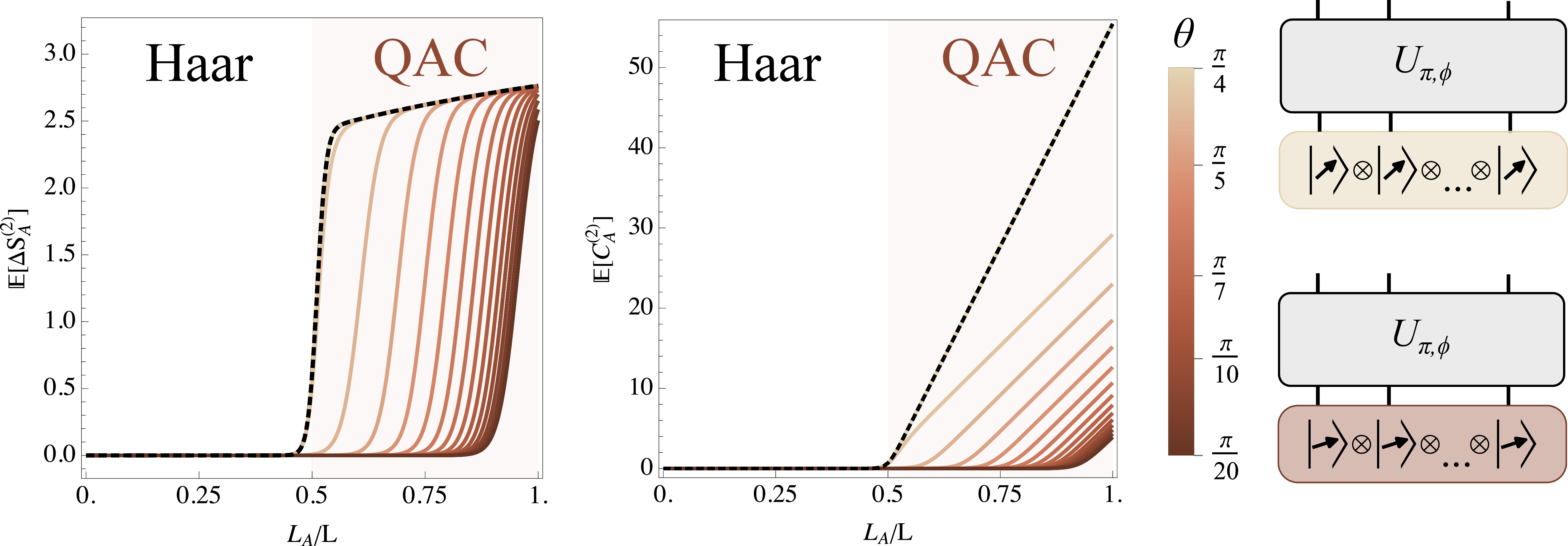
This work is organized in the following way. In section 2, we define the quantum automaton ensemble and recall some technical notions on the computation of entanglement asymmetry in random ensembles. We relegate to appendix A a more detailed presentation of the replica vectorization formalism for random quantum automata. In section 3, we compute the average Rényi-2 asymmetry of homogeneous product states and Dicke states in the random automaton ensemble. In section 4, we derive a closed set of equations for the time evolution of the Rényi-2 asymmetries of all subsystems and we present numerical solutions. We leave to appendix B the technical details of the derivation. In section 5, we present a decoupling inequality for the random automaton ensemble and explain the findings of the previous sections by looking at the connection between subsystem asymmetry and subsystem coherence. We conclude in section 6.
2 Preliminaries
In this section, we review some important notions concerning the quantum automaton ensemble and the entanglement asymmetry.
2.1 The quantum automaton ensemble
Throughout this paper, we consider a bipartite system with Hilbert space . The system consists of qubits in a lattice of arbitrary spatial dimension, thus the local Hilbert space is , , and:
| (2.1) |
with , , and .
The quantum automaton ensemble (QAE), denoted by , [26, 27] is the ensemble of operations with specified action on a basis of , which we choose to be the computational basis . Namely:
| (2.2) |
where is an element of the permutation group on elements and . The measure on the ensemble is the composition of the flat measure on the discrete permutation group and the uniform measure over copies of . In other words, this ensemble consists of all random (and uniformly chosen) permutations of the basis states, followed by independent and random phase transformations of the basis states.1 In section 4, we will consider the ensemble of random quantum automaton circuits (QACs). For a fixed circuit depth , we denote the corresponding ensemble by . We will focus on a circuit with non-local connectivity, where at each discrete time step two random qubits are coupled by a gate of the form (2.2). By taking a suitable continuous time limit of the dynamics induced by a QAC, as explained in section 4, the ensemble is well-defined, and it was shown in [32] that, as and the ensemble averages over approach their stationary values, the Rényi-2 bipartite entanglement entropies averaged over the ensembles and coincide. In section 4, we will show that this property holds also for the averaged Rényi-2 bipartite entanglement asymmetry.
Any operation of the form (2.2) on a state preserves its participation entropy [104–108]. As stated in the introduction, the participation entropy of a state measures its degree of localization with respect to a given basis of the Hilbert space. Namely, we define the Rényi- participation entropy of as:
| (2.3) |
where we introduced the inverse participation ratio of the state [109]:
| (2.4) |
To see that the operation (2.2) preserves , it is sufficient to write and compute:
| (2.5) |
where we used the fact that each permutation is invertible. In the rest of the paper, the Rényi-2 participation entropy will play a crucial role.
Let us now express the average subsystem purity of a state in the ensemble . To do so, we employ the Choi-Jamiołkowski (CJ) representation, or vectorization formalism [110]. We review the essential results below, leaving the derivations and further details to appendix A. First, for every site we define the following states in the replicated local Hilbert space :2
| (2.6) |
as well as , and we analogously define , . The above states are not normalized, as indeed when the dimension of the local Hilbert space is , the overlaps are:
| (2.7) |
In the CJ representation, the 2-replica operator is mapped to the state:
| (2.8) |
Let now and , with the unitary matrix drawn from a certain ensemble , e.g. the Haar random ensemble or the random QAE. With the above definitions, the purity of the state averaged over is expressed as follows:
| (2.9) |
To compute the average purity, one needs the expression of the expectation value , which depends on the ensemble :
-
For the Haar random ensemble:
(2.10) -
For :
Furthermore, it holds that:
| (2.12) |
From the above, it follows that if is the Haar random ensemble then:
| (2.13) |
which is a standard result that holds also in any 2-design ensemble [15, 25]. If instead , then [32]:
| (2.14) |
Remarkably, unlike the Haar random expression eq. (2.13), the subsystem purity averaged over (2.14) explicitly depends on the inverse participation ratio of the state , hence on some details of the initial state.
2.2 Entanglement asymmetry and charged partition functions
The Rényi- entanglement asymmetry of the state is defined as the relative entropy [54]:
| (2.15) |
where the charge counts the number of qubits in the local state , the symmetrized density matrix is , with being the projectors onto the charge eigenspaces of , and . As above, we consider a state and we are interested in the expectation value of , averaged over an ensemble :
| (2.16) |
where the approximate equality holds as long as there is a self-averaging property in the ensemble (which is true for the quantities of interest both in the Haar random ensemble and in the QAE). The expectation values can be computed via the charged partition functions:
| (2.17) |
with and the charge, restricted to subsystem .
We are interested in the two-replica case, . Here, setting , one has . In the CJ representation, the average of this quantity reads:
| (2.18) |
where we defined the state [78, 80] , . Physically, the state implements the insertion of the charge operators between two copies of . The overlaps of with the vectors in eq. (2.6) are:
| (2.19) |
3 Averaged entanglement asymmetry in the quantum automaton ensemble
In this section, we compute the averaged entanglement asymmetry in the ensemble . As anticipated in the Introduction, our results are markedly different from those found in the Haar random ensemble [78]. We consider two classes of states, the homogeneous product states and the Dicke states, characterized by a different scaling of the participation entropy with the system size , namely linear for the product states and logarithmic for the Dicke states. We show analytically how the profile of , as a function of the subsystem size , strongly depends on the participation entropy.
3.1 Computation of the asymmetry
We start by computing the expectation value of the charged partition function in the QAE, for a state . From the expression eq. (2.18), together with the overlaps eqs. (2.12), (2.19) one immediately obtains
| (3.1) |
Notice that , thus we recover the known result for the average subsystem purity eq. (2.14). Furthermore, by computing:
| (3.2) |
we obtain:
We can now study the asymptotic behaviour of as follows. Let us write:
| (3.4) |
We are interested in the regime in which and the ratios , are fixed and between 0 and 1 as . Since as , by substituting in the above expression, the ratio reads:
up to exponentially suppressed terms. Our goal is to find the subsystem size such that, in the limit of large and up to terms decaying exponentially in , is zero when , and it is an increasing function of when . In other words, is the subsystem size at which symmetrization ceases to occur in the thermodynamic limit. We call the onset value of the asymmetry, or symmetrization scale. To find the latter, we recall that . Moreover, as we show below, we consider states for which decays rapidly in . Therefore, the onset value is obtained by imposing that is an exponentially decreasing function of for . Recalling that the participation entropy is related to the participation ratio as , this happens when:
| (3.6) |
Equation (3.6) is our first main result: in the QAE, unlike the Haar random ensemble, the onset of the asymmetry can occur when the size of the subsystem is significantly larger than , depending on the participation entropy of the initial state. In fact, with this definition, for we obtain at leading order in :
| (3.7) |
whereas, for , , up to terms decaying exponentially in . This means in particular that in the limiting case when the participation ratio reaches its maximum value , there will be no onset of the asymmetry.
Let us now focus on two classes of initial states, for which , and thus , scales in different ways with the system size (see also the Supplemental material of [32]):
-
The homogeneous product states:
(3.8) for which the second inverse participation ratio is:
(3.9) i.e., for any , it is exponentially decreasing in the system size , thus is linear in . In particular, with maximum value at (the initial state is a state of the computational basis, or and the state has trivially zero asymmetry for any realization in the QAE) and minimum value at .
-
The Dicke states:
(3.10) where the sum is over the computational basis states such that the bitstring has fixed Hamming weight , i.e. it contains exactly 1’s and 0’s. The second inverse participation ratio is:
(3.11) i.e. it has a power-law decay in the system size for : .
Of course, one could consider other states with different scaling behaviours of the participation entropy. For instance, the GHZ state has a constant inverse participation ratio . However, the two examples considered here suffice to illustrate our main results.
We now focus on the homogeneous product state. Up to terms decaying exponentially in , eq. (3.7) becomes
| (3.12) |
which reproduces the asymptotic behavior of the average Rényi-2 asymmetry in the Haar random ensemble when the subsystem size is [78]. Moreover, from the expression eq. (3.9), we can obtain the values of the tilting angle for which the onset of the asymmetry is at . This happens when , that is when (for ):
| (3.13) |
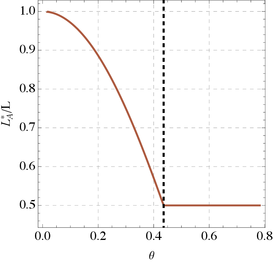
Note that . This phenomenology is quite surprising, as the specific scaling of the participation entropy for these states indicates that there is a critical angle below which the onset of the asymmetry changes from the typical value to . The averaged entanglement asymmetry as a function of the subsystem size for different homogeneous product states is shown in figure 2, together with the finite-size scaling of the results for a fixed value of the tilting parameter . The values of as a function of are shown in figure 4.
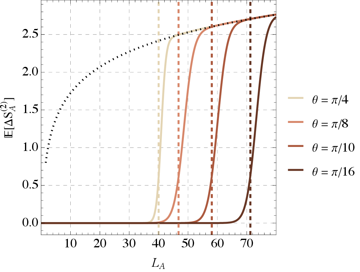
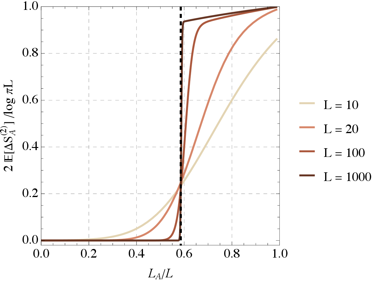
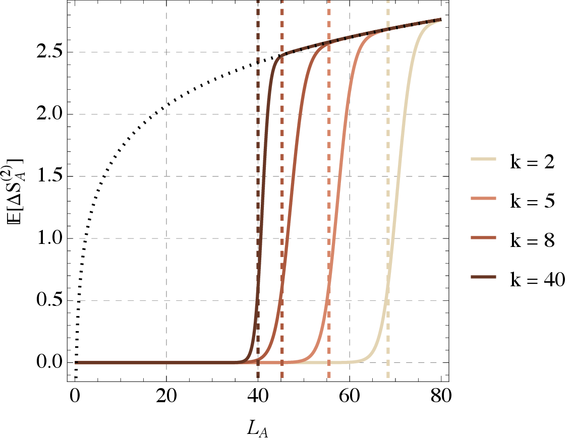
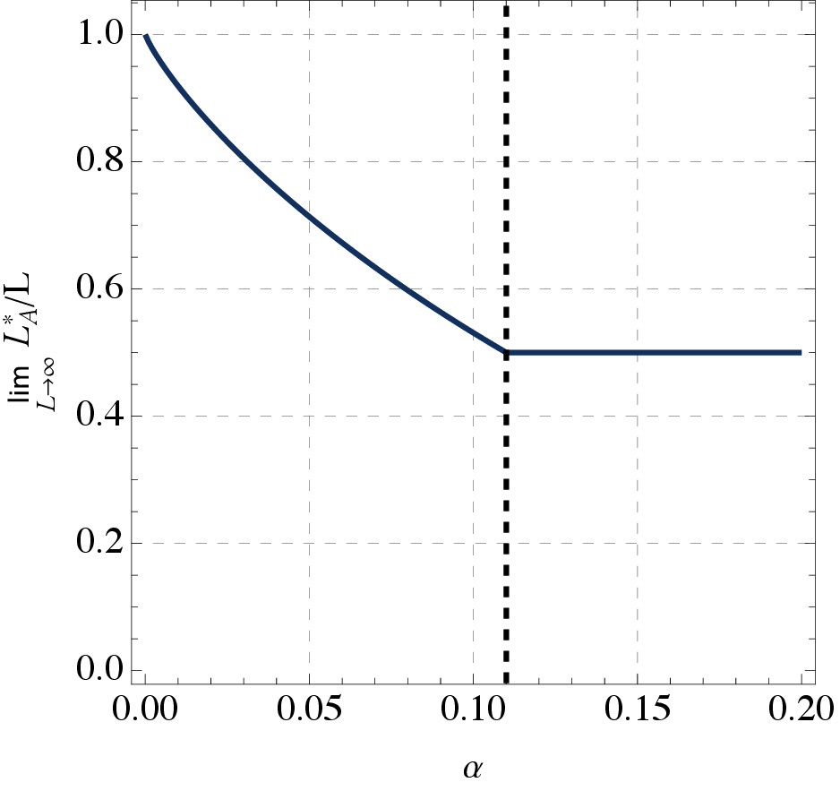
For the Dicke state , eq. (3.7) yields the same leading order term of eq. (3.12), but with a power-law decaying correction . The averaged entanglement asymmetry Page-curve for different values of and is shown in figure 3. Interestingly, unlike the case of homogeneous product states where the critical angle does not depend on the system size, for the states the critical value of at which the onset value shifts from the typical value to depends on the system size. This is due to the different scaling of the participation entropy with the system size . In the large limit, letting , we can approximate
| (3.14) |
where is the binary entropy and we used Stirling’s formula . Restricting ourselves to values of , we arrive at the critical value of for which :
| (3.15) |
That is, the shift in the symmetrization scale happens for Dicke states with , as shown in figure 4.
4 Dynamics of entanglement asymmetry in a two-local quantum automaton circuit
In this section, we study the dynamics of the averaged Rényi-2 entanglement asymmetry under a non-local quantum circuit evolution, starting from a homogeneous product state. In particular, we consider a 2-local quantum circuit, that is, at any time step, with a certain probability a 2-body gate , consisting of a permutation of basis states followed by a global phase transformation is applied to two qubits in random sites and . A slight generalization of this protocol was employed in [100] to study the dynamics of the averaged Rényi-2 entropy under a 2-local random unitary circuit (RUC). The same protocol we study here was followed in [80] to compute the averaged Rényi-2 asymmetry in the Haar random case, and the averaged Rényi-2 entropy in the case of random permutation circuits and random quantum automata in [32].
The advantage with respect to a local (brickwork) circuit, which requires mapping the system to a classical statistical model to obtain analytical predictions [3, 15, 18, 80], is that with a non-local protocol one can construct a set of observables with a Markovian evolution, governed by a system of differential equations. By numerically solving these differential equations, the expectation values of the charged moments at any time for all subsystem sizes are obtained at once, as well as the expectation values of the subsystem purities. As we will discuss in section 5, from the same system of differential equations one can also extract the average coherence of all subsystems.
4.1 Differential equations for the charged moments
In a 2-local quantum circuit, at each discrete time step , with a certain probability we apply a two-body gate , , to the state , so that at time the state is , where with probability , and with probability . At time , is the identity operator. Then, we average over the sites (chosen with uniform probability) and over the ensemble from which the operators are drawn, that is the quantum automaton circuit ensemble (QAC). In the continuous time limit (see appendix A of [100]), this evolution protocol yields a master equation for the two-replica average :
| (4.1) |
with
| (4.2) |
The expectation value can be obtained in the very same way as the corresponding expectation value in the global ensemble QAE (see appendix A), with the only difference that now is an operator acting non-trivially only on the replica Hilbert space . Thus, by replacing in eq. (2.11) with , we have:
where we introduced the notation for .
The averaged time-dependent charged moment is given by:
| (4.4) |
and its time derivative is:
| (4.5) |
If the right-hand side of the above equation was a linear combination of the averaged moments for different subsystems , one would have a complete system of equations for the time evolution of the charged moments of all subsystems. However, this is not the case, because the action of on produces extra terms other than a linear combination of states for different (complementary) subsystems and , even if one considers a simpler RUC [80]. In order to obtain a closed set of equations, we notice that the Lindbladian is invariant under site permutation. If one also chooses a permutation-invariant initial state, such as the homogeneous product states eq. (3.8), then the (averaged) state at any is site-permutation invariant. In this scenario, a closed set of equations is obtained by introducing the following states:
| (4.6) |
In the above expression, the indices , , and are non-negative integers such that , is a permutation of the sites and implements that permutation on the states. Thus, is the permutation-invariant state in the two-replica space containing copies of the state and so on for the other indices. This is a generalization of the states introduced in [32] to compute the averaged purity in non-local QACs, and of the states introduced in [80] to compute the averaged asymmetry in non-local RUCs.
It is easy to derive the action of the operators on any state. The following relations can be found in [32]:
We then need to evaluate the action of on the states with at least one factor . This is easily done by using the overlaps in eqs. (2.19), and we obtain:
with
Since , and eqs. (4.8) reduce to (4.7) when .
Following [32], we want to write a system of ODEs for the functions
| (4.10) |
with the convention that is zero whenever any of the indices is smaller than zero or larger than . Since there are of these functions, corresponding to the number of tuples of non-negative integers such that , the number of independent equations in the system is . These are obtained from the Lindbladian operator in eq. (4.2):
| (4.11) |
together with eqs. (4.7) and (4.8). Leaving the details of the derivation to appendix B, we obtain:
| (4.12) |
with
the only non-vanishing coefficients. Thus, all the functions evolve with a closed system of linear ODEs. In particular, for permutation-invariant initial states, the average charged moments of a subsystem are functions only of the subsystem size . Indeed, we can rewrite eq. (4.4) as:
| (4.14) |
The evolution equation for can be read-off from eq. (4.12):
We notice that, when the equations (4.12) reduce to those derived in [32] for the evolution of the average subsystem purity in a QAC, i.e. a complete system of equations for the functions . Remarkably, by solving this system, one obtains as a byproduct the dynamics of the relative entropy of coherence for all subsystems. We show how this is done in appendix B.
We now need to establish the initial conditions for the functions , i.e.:
| (4.16) |
where and is the homogeneous product state eq. (3.8). It follows from the definition eq. (2.8) that we can write (see also the Supplemental material of [32]):
| (4.17) |
Since is a permutation invariant state, one easily obtains:
As a sanity check, let us consider some specific initial conditions in detail. When , one has as expected, since the initial state is a product state. On the other hand, the quantity reproduces the second inverse participation ratio of , eq. (3.9). Finally, Although the time-dependent averaged asymmetry can only be obtained numerically by integrating over , the Rényi-2 asymmetry of can be obtained in the following way:
where we used the result eq. (3.2), which is the same when the function is replaced by in the integrand, and the standard definition of the Hypergeometric function [111]. The above result (4.19) was first obtained, for a generic number of replicas, in [54].
We conclude by observing that, even though finding the analytical solution to the system of equations (4.12) is extremely challenging, the stationary solutions to the latter, obtained by imposing , are much easier to find. Indeed, these are given by the following functions:
| (4.20) |
The expectation value in the above expression is taken in the global QAE, and indeed the quantities are simple generalizations of the expression eq. (3.1), and they can be computed with the same techniques used in section 3. Explicitly:
| (4.21) |
where and . A direct substitution into eq. (4.12) shows that these functions yield a steady-state solution of the system. This proves that the ensemble averages of the Rényi-2 entanglement asymmetry computed in and coincide, at any finite size .
4.2 Numerical results
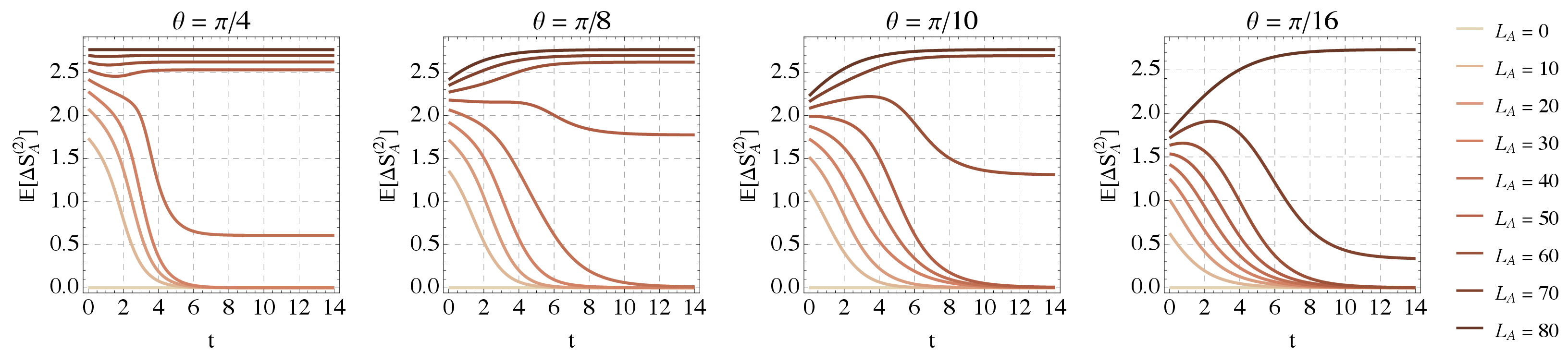
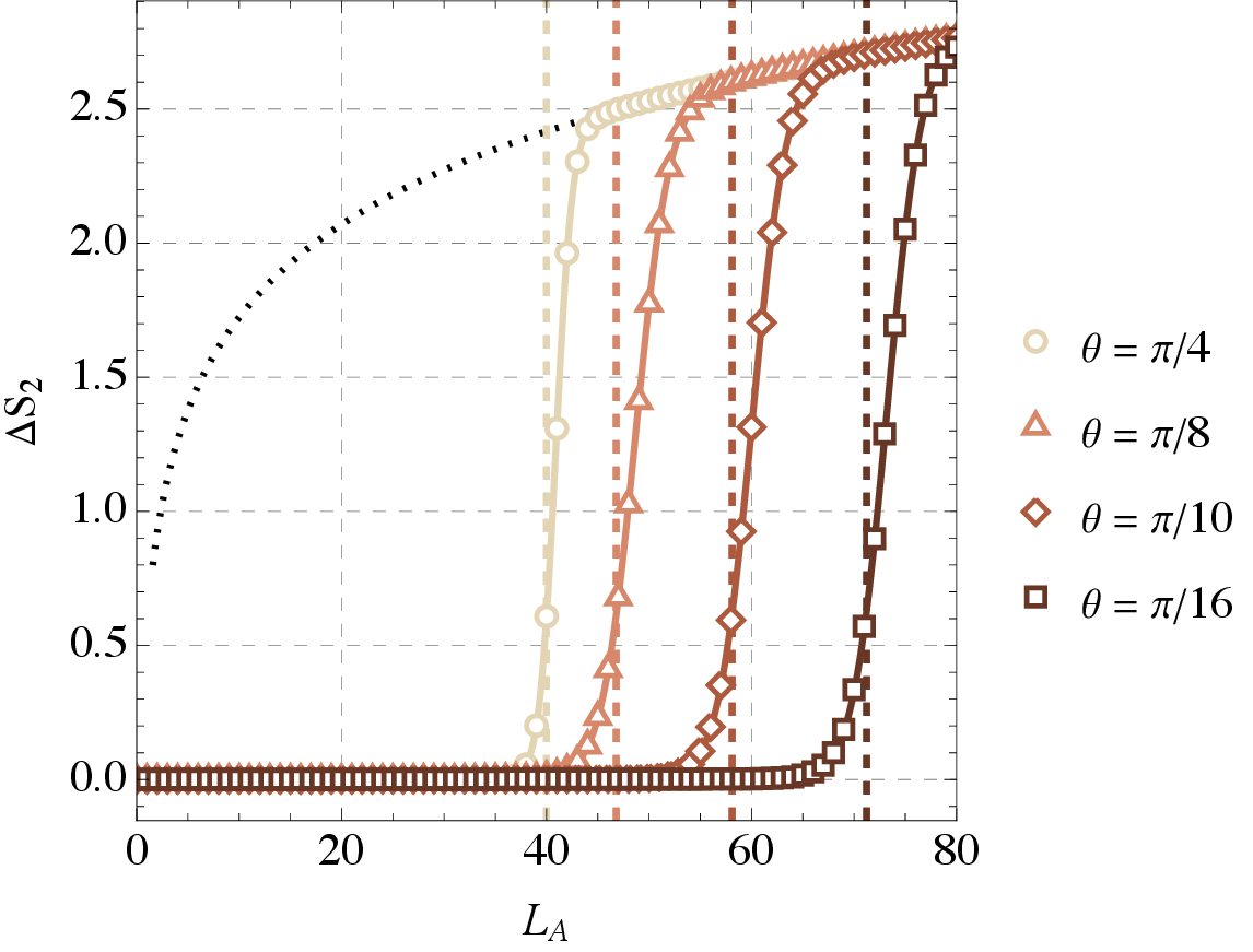
We now discuss the time evolution of the averaged entanglement asymmetry under the 2-local random quantum automaton circuit evolution, shown in figure 5. The results are obtained through numerical integration of eq. (4.12), following the outline of this section. The system is initialized in a homogenous product state (3.8) for different values of the tilting angle . We set the system size , and run the evolution until the asymmetry reaches their stationary value. As apparent from figure 5, curves corresponding to different subsystem sizes relax to either a finite value or zero, depending on the specific choice of and . The extracted stationary values are plotted against the subsystem size in figure 6, together with the global results (3.3). As expected, the long-time local results match the global ones: the asymmetry stays zero for subsystem sizes , then rapidly increase to the value . The onset point is the same as for the global case, given in eq. (3.6).
5 Connection to subsystem coherence
In this section, we provide a justification for the results presented in the previous sections. In particular, we give a physical argument as to why in the QAE the onset of the averaged asymmetry may occur at subsystem sizes much larger than . Essentially, we show that a very small participation entropy (equivalently, a very high degree of localization in the Hilbert space) prevents the build-up of subsystem coherence up to a subsystem size precisely given by eq. (3.6). This complements the picture presented in [32], where it was shown that a small participation entropy prevents entanglement saturation to a volume law at large subsystem sizes. First, we discuss the distinguishability between the subsystem’s density matrix and the infinite-temperature state in the ensemble of random quantum automata. Namely, we generalize the decoupling inequality first derived in [1]. The decoupling inequality explains why symmetrization occurs at small subsystem sizes, but it is not enough to infer the value in eq. (3.6). Therefore, we propose a criterion for the onset of asymmetry based on the notion of subsystem coherence and use it to explain the findings of the previous sections.
5.1 The decoupling inequality
We prove an upper bound (decoupling inequality) on the averaged squared trace distance between the state and the maximally mixed state on , where the average is over . Let us recall some preliminary definitions (see e.g. [110]). Let be the space of linear operators over , and . The Schatten -norm of is defined as:
| (5.1) |
We are interested in Schatten norms with . For this is the trace norm, which coincides with the sum of the singular values of : . For , the Schatten norm is the Hilbert-Schmidt (HS) norm, induced by the HS inner product . The Schatten norm satisfies the following Hölder inequality. For every :
| (5.2) |
In particular, take in the above inequality, and take . Then, since , . Thus, the Holder inequality reads:
| (5.3) |
The decoupling inequality is easily obtained from the inequality (5.3). In fact, considering a bipartite Hilbert space as in (2.1), in order to bound the trace distance between and the completely mixed state , we define and apply the above inequality (squared) to :
| (5.4) |
The above decoupling inequality holds in full generality. Suppose that , for some initial state , and the unitary matrix is drawn from some ensemble . Then:
| (5.5) |
For the Haar random ensemble, from eq. (2.13) it follows
| (5.6) |
which is the inequality presented in [78, 80].
On the other hand, for , from eq. (2.14) it follows that:
| (5.7) |
implying the decoupling inequality:
| (5.8) |
Keeping , fixed in the large- limit, the right-hand side of the above inequality reads
| (5.9) |
where, as usual, the symbol means that the two terms differ by a quantity exponentially small in . Therefore, on average, the trace distance between and the completely mixed state in is exponentially small as long as:
| (5.10) |
We remark that the decoupling inequality is stated using the trace distance, rather than the HS distance, as only the former has a clean interpretation in terms of distinguishability of quantum states [110, 112].
The decoupling inequality for the QAE, eq. (5.8), explains the Page curve for the average Rényi-2 entropy in this ensemble (as well as the 2-local circuit Page curve) found in [32] (cfr. figure 1.b of the Supplemental material): for subsystems smaller than half the total system, when , the average Rényi-2 entropy saturates to the constant value . This allows us to interpret the quantity as the effective support of the state , which coincides with the actual support if and only if has uniform weights over basis states. Naively, the condition (5.10) means that when the effective support , the state can be, on average, exponentially close in trace distance to the maximally mixed state in only as long as .
Since the fully mixed state is -invariant, the decoupling inequality also explains why when (5.10) holds. However, the asymmetry remains zero also at larger subsystem sizes, namely for , see eq. (3.6). When is larger than the right-hand side of eq. (5.10), the decoupling inequality does not explain the behaviour of the asymmetry. In the following section, we argue that the onset of the asymmetry happens when the subsystem coherence starts to become relevant. This is our second main result.
5.2 Coherence and asymmetry onset
In order to provide a criterion for the asymmetry onset, we turn now to the study of the average coherence content of the reduced density matrix. In particular, we are interested in estimating how much departs from being diagonal in the computational basis of . To do so, we define the fully dephasing channel with respect to that basis, and the dephased subsystem density matrix:
| (5.11) |
Intuitively, the onset of coherence in subsystem occurs when the norm of the diagonal matrix is comparable to the norm of the matrix , consisting of all and only the off-diagonal elements in the computational basis. Thus, we want to compare the norms and . Notice that the dephased state is obviously closer to (in HS norm) than the fully mixed state, and in particular:
| (5.12) |
where the strict equality follows from the fact that the two states and are orthogonal in the HS product, since the first has no diagonal entries and the second is diagonal.3
Based on the above intuition, we define the onset of the average subsystem coherence in the ensemble as the size such that, for , one has:
| (5.13) |
up to terms exponentially small in the total system size . In principle, the coherence onset does not need to happen at the same subsystem size where we observe the asymmetry onset. Indeed, for any reduced density matrix , one can write , where the two matrices both have only off-diagonal elements in the computational basis, but the only non-zero entries of are between states belonging to the same charge sector, and the only non-zero entries of are between states belonging to different charge sectors. A state with but is not coherent, but it is -symmetric, hence the onset of coherence can never occur at larger system sizes with respect to the onset of asymmetry. In our case, because the state is evolved with a random operation that does not preserve the charge, and because the average is performed with a uniform distribution over all the possible permutations and phase transformation, we do not expect any “preference” in the onset of the off-diagonal entries. In other words, we expect the onset of coherence to coincide with the onset of asymmetry, . The spread of coherence under -preserving Haar random dynamics was recently studied in [41].
Now, in eq. (5.13), we can compute:
| (5.14) |
where in the second equation, we used the fact that . The purity of is expressed in the CJ representation as follows (see appendix A and [41]):
| (5.15) |
hence the average over an ensemble of the above quantity is:
| (5.16) |
Notice that the only difference with respect to the CJ expression of the purity of , eq. (2.9), is that the 2-replica state is replaced by , the CJ representation of the dephasing operator in subsystem . Thus, in the random quantum automaton ensemble:
| (5.17) |
and
| (5.18) |
Again, in the above expressions, the second approximate equality holds up to exponentially decreasing terms in the system size. In the case of homogeneous product states eq. (3.8) with , for which is an exponentially decreasing function of , one has the further asymptotic approximations:
| (5.19) |
Therefore, in the large- limit, the onset condition for coherence, eq. (5.13), is verified if:
| (5.20) |
which is precisely equivalent to the asymmetry onset condition eq. (3.6).
The quantity is strictly related to the subsystem’s Rényi-2 relative entropy of coherence [41]:
| (5.21) |
Notice that, for the full system, since the state is pure, one has:
| (5.22) |
that is, the total system’s coherence coincides with its participation entropy (this is of course true also for higher Rényi entropies as well as for the von Neumann entropy of coherence). In particular, for any realization of the operations in the QAE, equals the second participation entropy of the initial state, and thus it is conserved by the dynamics.
On the other hand, from the above discussion, it follows that the average subsystem’s Rényi-2 entropy of coherence is zero for and starts to grow linearly for , with subleading corrections around , given by eq. (3.6). To see that this is the case, notice that eq. (5.17) implies:
| (5.23) |
while the expression for the averaged purity, eq. (2.14), yields (see also [32]):
| (5.24) |
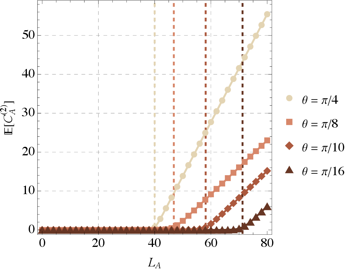
We plot the quantity for different homogeneous product states in figure 7, as a function of and see very clearly both the distinct onset values depending on and the subsequent linear growth.
We conclude by observing that the dynamics of the average subsystem coherence in the 2-local QAC described in section 4 can be extracted from the same equations ruling the dynamics of the average asymmetry. To be precise, one does not need the full system of ODEs (4.12) to obtain the time evolution of the average coherence, as it is sufficient to obtain a solution for the functions obtained by setting . We provide some details and numerical results in appendix B.
6 Discussion and outlook
We have studied the average subsystem -asymmetry in quantum automaton ensembles with two different underlying geometries, corresponding to a global all-to-all transformation and a 2-local circuit. We have shown that the global ensemble average of the asymmetry coincides with the late-time limit of the circuit result at any system size. In a 2-local quantum automaton circuit, contrary to the random unitary case, the symmetrization of a subsystem under the dynamics occurs until subsystem’s size reaches a value that depends on the initial state, namely on its participation entropy. We have derived a closed formula for this scale and quantified it for different classes of initial states. The scale at which subsystem symmetrization ceases to happen cannot be derived solely by looking at the averaged quantum distance between the reduced density matrix and the fully mixed state. Indeed, we have connected the emergence of this symmetrization scale to the growth of the average subsystem coherence and showed that they share the same characteristic length scale. Our work highlights the sharp differences between “traditional” random unitary circuits and random quantum automata and reveals interesting new quantum phenomena.
There are several open questions raised by our work. First, it would be important to study the dynamics of entanglement asymmetry in random permutation circuits, which, on top of preserving the initial state participation entropy, display an isolated non-thermal stationary state. The tools needed to extend our results to random permutation circuits are the same applied here, although the analytical treatment of random permutations without random phases is significantly more demanding. Furthermore, since quantum automaton circuits can be implemented on current quantum platforms, investigating the growth of other relevant resources in this setting, such as nonstabilizerness and non-Gaussianity, would be extremely timely. Finally, another natural direction is to include forms of monitoring in the random automaton evolution, and see how the late time Page-curves of entanglement, asymmetry and other quantum resource monotones are affected by monitoring.
Acknowledgments
MM and DSS would like to thank Filiberto Ares, Sara Murciano, Pasquale Calabrese and especially Lorenzo Piroli for fruitful discussions. This work was funded by the European Union (ERC, QUANTHEM, 101114881). Views and opinions expressed are however those of the author(s) only and do not necessarily reflect those of the European Union or the European Research Council Executive Agency. Neither the European Union nor the granting authority can be held responsible for them.
Appendix
A Choi-Jamiołkowski representation for random quantum automata
In this appendix, we derive some results on the Choi-Jamiołkowski representation for the random QAE which are used in the main text.
A.1 Purities in the Choi-Jamiołkowski representation
Let be a (finite-dimensional) Hilbert space with a basis . The identity, swap and dephasing operators in the two-replica space are:
| (A.1) |
For any one-replica operator , , the following identities hold:
where in the last equation, we used the one-replica expression of the dephasing operator: . In particular, for two copies of the same density matrix :
| (A.5) |
where and is the second inverse participation ratio in the basis .
Consider now a bipartite space , with a basis . We define the two-replica operators and , respectively acting as the swap and dephasing operator in , and as the identity in :
| (A.6) |
with the convention that , where is in the first copy of , and is in the second. Thus, the purity of the reduced density matrix , and the purity of the dephased reduced density matrix can be expressed as:
The Choi-Jamiołkowski isomorphism [110] is a linear map that associates a state to any completely positive operator. In particular, in one replica, it is a map from to , and the density matrix operator is mapped to:
| (A.9) |
that is, is the un-normalized maximally entangled state in , which represents the identity. If is the tensor product of local Hilbert spaces , then . It is straightforward to check that in this formalism , and in particular . The isomorphism is easily extended to the case where there are more replicas of the original Hilbert space. in particular, for two replicas, the isomorphism becomes a map from to and:
| (A.10) |
where we adopt the same notation to represent the tensor product of two fully entangled states in two copies of :
| (A.11) |
In general, it will be clear from the context whether is a state in or in . The swap and the dephasing operators are mapped to:
| (A.12) |
as one can immediately check that:
| (A.13) |
If there is a spatial bipartition then, defining , it is also easy to check:
| (A.14) |
Combining the above equations with eqs. (A.7) and (A.8), we obtain the expression of the purities and in the Choi-Jamiołkowski representation:
| (A.15) |
A.2 First and second moments
In this appendix, we compute the expectation values and , where are drawn from the random quantum automaton ensemble . Here, denotes the complex conjugate of . First, let us recall the useful identity for the Choi-Jamiołkowski representation of a product:
| (A.16) |
which holds for every completely positive operator , , . It is easy to see that the above is true, as for on one hand:
| (A.17) |
and on the other hand:
| (A.18) |
Thus, in particular, for a state , in one and two replicas the following holds:
| (A.19) |
Let us then compute the moments:
| (A.20) |
where, concretely, the average is over the set of random phases and random permutations of the computational basis states.
Let us consider . On a computational basis state , :
| (A.21) |
for some permutation and some , thus on a basis state :
| (A.22) |
The average over the phases selects . In fact, if then the phases are independent and . Then, the average over permutations is the sum over of , divided by the total number of permutations, which is . For every label , there are exactly permutations that keep fixed. Thus:
| (A.23) |
yielding:
| (A.24) |
which in operatorial form is the fully mixed state .
We now compute . On a basis state , the action of reads:
| (A.25) |
The average over the phases yields a nonzero contribution if the sets , which happens in three distinct cases: , or , or . Consider first the case . This computation is completely analogous to that of :
| (A.26) |
Next, consider the case , where . Because the permutation is a bijection, if then , and there are out of the total permutations that map the pair to , with . Thus, for :
| (A.27) |
The case is analogous to the one above, leading to (for ):
| (A.28) |
Putting everything together:
which is exactly eq. (2.11) in the main text.
We mention that the above expectation values, eqs. (A.24) and (A.29), can also be deduced from the Weingarten matrix of the random permutation ensemble [28] by selecting, among the invariant 2-replica states in that ensemble, those which are also invariant under random phase transformations.
B Details on the dynamics in non-local QAC
In this section, we provide the details of the derivation of eq. (4.12), which closely follows the derivation of the analogous system for the averaged subsystem purities in the Supplemental material of [32].
B.1 Derivation of the differential equations for the charged moments
We start by explicitly writing the action of the permutation operator in eq. (4.6) as follows:
| (B.1) |
where , , , . In order to evaluate the action of on , for each permutation we split the sum over and in the following way:
We can now proceed exactly as in [32], using the relations (4.7) and (4.8):
Adding to the above the contribution coming from the identity in eq. (4.2) and taking the overlap with , we end up with the following differential equation:
which reproduces eq. (4.12).
B.2 Dynamics of the averaged purity and Rényi-2 entropy of coherence
As mentioned in section 4, the dynamics of the average purities of all subsystems can be obtained by solving a simpler, closed set of equations for the functions . This system was derived in [32], and we report it below:
For a permutation invariant initial state, the average purity at time , is the same for all subsystems such that and it is given by .
Remarkably, once the system eq. (B.5) is solved, as a byproduct one also obtains all the average Rényi-2 entropies of coherence. To be precise, from the definition eq. (5.15) and using permutation invariance, we find that:
| (B.6) |
and in particular , . The time-profile of the average Rényi-2 entropy of coherence, see eq. (5.21), can be then obtained using the self-averaging properties of the QAC ensemble:
| (B.7) |
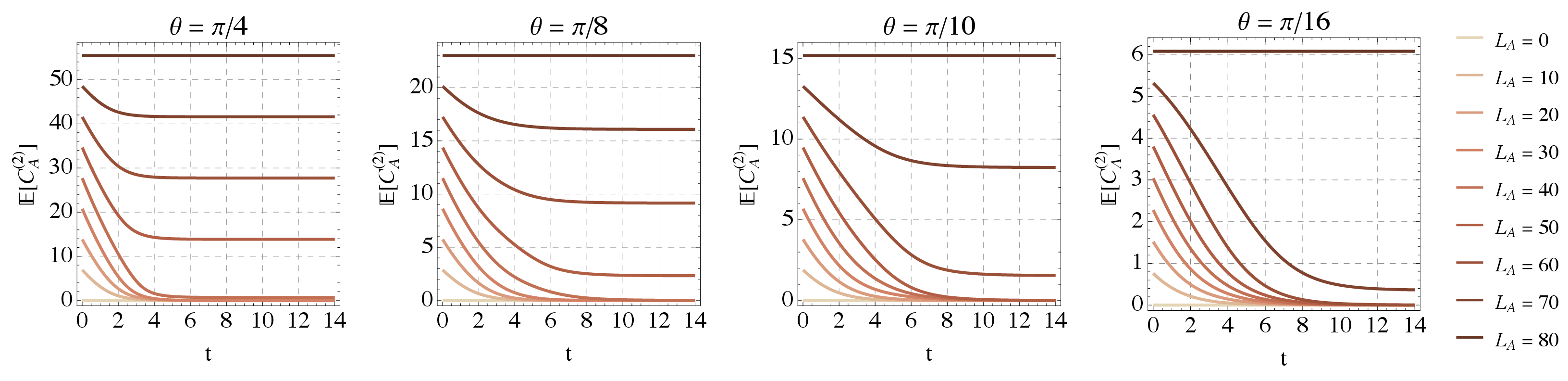
The numerical results for the time-evolution of the average subsystem coherence, starting from an homogeneous product state, are shown in figure 8.
Funding Statement. This paper has been funded by the following grants/awards. European Research Council: StG QUANTHEM, 10111488.
Data Availability Statement. My article has associated data in a repository Available at: https://amsacta.unibo.it.
Open Access. This article is distributed under the terms of the Creative Commons Attribution License (CC-BY4.0), which permits any use, distribution and reproduction in any medium, provided the original author(s) and source are credited.
References
- [1]
- P. Hayden and J. Preskill, Black holes as mirrors: Quantum information in random subsystems, JHEP 09 (2007) 120 [arXiv:0708.4025] [INSPIRE].
- [2]
- B. Bertini, P. Kos and T. Prosen, Exact Correlation Functions for Dual-Unitary Lattice Models in 1+1 Dimensions, Phys. Rev. Lett. 123 (2019) 210601 [arXiv:1904.02140] [INSPIRE].
- [3]
- A. Nahum, J. Ruhman, S. Vijay and J. Haah, Quantum Entanglement Growth Under Random Unitary Dynamics, Phys. Rev. X 7 (2017) 031016 [arXiv:1608.06950] [INSPIRE].
- [4]
- T. Zhou and A. Nahum, Emergent statistical mechanics of entanglement in random unitary circuits, Phys. Rev. B 99 (2019) 174205 [arXiv:1804.09737] [INSPIRE].
- [5]
- B. Bertini, P. Kos and T. Prosen, Entanglement spreading in a minimal model of maximal many-body quantum chaos, Phys. Rev. X 9 (2019) 021033 [arXiv:1812.05090] [INSPIRE].
- [6]
- S. Gopalakrishnan and A. Lamacraft, Unitary circuits of finite depth and infinite width from quantum channels, Phys. Rev. B 100 (2019) 064309 [arXiv:1903.11611] [INSPIRE].
- [7]
- T. Zhou and A. Nahum, Entanglement Membrane in Chaotic Many-Body Systems, Phys. Rev. X 10 (2020) 031066 [arXiv:1912.12311] [INSPIRE].
- [8]
- A. Foligno, P. Kos and B. Bertini, Quantum Information Spreading in Generalized Dual-Unitary Circuits, Phys. Rev. Lett. 132 (2024) 250402 [arXiv:2312.02940] [INSPIRE].
- [9]
- L. Piroli, B. Bertini, J.I. Cirac and T. Prosen, Exact dynamics in dual-unitary quantum circuits, Phys. Rev. B 101 (2020) 094304 [arXiv:1911.11175] [INSPIRE].
- [10]
- K. Klobas, B. Bertini and L. Piroli, Exact Thermalization Dynamics in the “Rule 54” Quantum Cellular Automaton, Phys. Rev. Lett. 126 (2021) 160602 [arXiv:2012.12256] [INSPIRE].
- [11]
- B. Bertini, C. De Fazio, J.P. Garrahan and K. Klobas, Exact Quench Dynamics of the Floquet Quantum East Model at the Deterministic Point, Phys. Rev. Lett. 132 (2024) 120402 [arXiv:2310.06128] [INSPIRE].
- [12]
- H.-R. Wang, X.-Y. Yang and Z. Wang, Exact Hidden Markovian Dynamics in Quantum Circuits, Phys. Rev. Lett. 133 (2024) 170402 [arXiv:2403.14807] [INSPIRE].
- [13]
- P. Hosur, X.-L. Qi, D.A. Roberts and B. Yoshida, Chaos in quantum channels, JHEP 02 (2016) 004 [arXiv:1511.04021] [INSPIRE].
- [14]
- C. von Keyserlingk, T. Rakovszky, F. Pollmann and S. Sondhi, Operator hydrodynamics, OTOCs, and entanglement growth in systems without conservation laws, Phys. Rev. X 8 (2018) 021013 [arXiv:1705.08910] [INSPIRE].
- [15]
- A. Nahum, S. Vijay and J. Haah, Operator Spreading in Random Unitary Circuits, Phys. Rev. X 8 (2018) 021014 [arXiv:1705.08975] [INSPIRE].
- [16]
- P.W. Claeys and A. Lamacraft, Maximum velocity quantum circuits, Phys. Rev. Res. 2 (2020) 033032 [arXiv:2003.01133] [INSPIRE].
- [17]
- B. Bertini and L. Piroli, Scrambling in Random Unitary Circuits: Exact Results, Phys. Rev. B 102 (2020) 064305 [arXiv:2004.13697] [INSPIRE].
- [18]
- M.P.A. Fisher, V. Khemani, A. Nahum and S. Vijay, Random Quantum Circuits, Ann. Rev. Condens. Mat. Phys. 14 (2023) 335 [arXiv:2207.14280] [INSPIRE].
- [19]
- N. Hunter-Jones, Unitary designs from statistical mechanics in random quantum circuits, arXiv:1905.12053 [INSPIRE].
- [20]
- A.M. Dalzell, N. Hunter-Jones and F.G.S.L. Brandão, Random Quantum Circuits Anticoncentrate in Log Depth, PRX Quantum 3 (2022) 010333 [arXiv:2011.12277] [INSPIRE].
- [21]
- A.W. Harrow and S. Mehraban, Approximate Unitary t-Designs by Short Random Quantum Circuits Using Nearest-Neighbor and Long-Range Gates, Commun. Math. Phys. 401 (2023) 1531 [arXiv:1809.06957] [INSPIRE].
- [22]
- S. Mittal and N. Hunter-Jones, Local random quantum circuits form approximate designs on arbitrary architectures, arXiv:2310.19355 [INSPIRE].
- [23]
- T. Schuster, J. Haferkamp and H.-Y. Huang, Random unitaries in extremely low depth, Science 389 (2025) adv8590 [arXiv:2407.07754] [INSPIRE].
- [24]
- N. LaRacuente and F. Leditzky, Approximate Unitary k-Designs from Shallow, Low-Communication Circuits, Commun. Math. Phys. 407 (2026) 51 [arXiv:2407.07876] [INSPIRE].
- [25]
- A.A. Mele, Introduction to Haar Measure Tools in Quantum Information: A Beginner’s Tutorial, Quantum 8 (2024) 1340 [arXiv:2307.08956] [INSPIRE].
- [26]
- J. Iaconis, A. Lucas and X. Chen, Measurement-induced phase transitions in quantum automaton circuits, Phys. Rev. B 102 (2020) 224311 [arXiv:2010.02196] [INSPIRE].
- [27]
- J. Iaconis, Quantum State Complexity in Computationally Tractable Quantum Circuits, PRX Quantum 2 (2021) 010329 [arXiv:2009.05512] [INSPIRE].
- [28]
- B. Bertini, K. Klobas, P. Kos and D. Malz, Quantum and Classical Dynamics with Random Permutation Circuits, Phys. Rev. X 15 (2025) 011015 [arXiv:2407.11960] [INSPIRE].
- [29]
- S. Gopalakrishnan and B. Zakirov, Facilitated quantum cellular automata as simple models with non-thermal eigenstates and dynamics, Quantum Sci. Technol. 3 (2018) 044004 [arXiv:1802.07729] [INSPIRE].
- [30]
- S. Gopalakrishnan, Operator growth and eigenstate entanglement in an interacting integrable Floquet system, Phys. Rev. B 98 (2018) 060302 [arXiv:1806.04156] [INSPIRE].
- [31]
- B. Bertini, K. Klobas, P. Kos and D. Malz, Random permutation circuits beyond qubits are quantum chaotic, Phys. Rev. B 113 (2026) L100302 [arXiv:2508.10890] [INSPIRE].
- [32]
- D. Szász-Schagrin et al., Entanglement dynamics and Page curves in random permutation circuits, Phys. Rev. Res. 8 (2026) L012061 [arXiv:2505.06158] [INSPIRE].
- [33]
- E. Chitambar and G. Gour, Quantum resource theories, Rev. Mod. Phys. 91 (2019) 025001 [arXiv:1806.06107] [INSPIRE].
- [34]
- C.H. Bennett, H.J. Bernstein, S. Popescu and B. Schumacher, Concentrating partial entanglement by local operations, Phys. Rev. A 53 (1996) 2046 [quant-ph/9511030] [INSPIRE].
- [35]
- C.H. Bennett, D.P. DiVincenzo, J.A. Smolin and W.K. Wootters, Mixed state entanglement and quantum error correction, Phys. Rev. A 54 (1996) 3824 [quant-ph/9604024] [INSPIRE].
- [36]
- R. Horodecki, P. Horodecki, M. Horodecki and K. Horodecki, Quantum entanglement, Rev. Mod. Phys. 81 (2009) 865 [quant-ph/0702225] [INSPIRE].
- [37]
- V. Vedral, M.B. Plenio, M.A. Rippin and P.L. Knight, Quantifying entanglement, Phys. Rev. Lett. 78 (1997) 2275 [quant-ph/9702027] [INSPIRE].
- [38]
- T. Baumgratz, M. Cramer and M.B. Plenio, Quantifying Coherence, Phys. Rev. Lett. 113 (2014) 140401 [arXiv:1311.0275] [INSPIRE].
- [39]
- A. Streltsov, G. Adesso and M.B. Plenio, Quantum Coherence as a Resource, Rev. Mod. Phys. 89 (2017) 041003 [arXiv:1609.02439] [INSPIRE].
- [40]
- G. Saxena, E. Chitambar and G. Gour, Dynamical resource theory of quantum coherence, Phys. Rev. Res. 2 (2020) 023298 [arXiv:1910.00708] [INSPIRE].
- [41]
- S. Aditya, E. Tirrito, P. Sierant and X. Turkeshi, Coherence dynamics in quantum many-body systems with conservation laws, arXiv:2604.23192 [INSPIRE].
- [42]
- X. Turkeshi and P. Sierant, Hilbert Space Delocalization under Random Unitary Circuits, Entropy 26 (2024) 471 [arXiv:2404.10725] [INSPIRE].
- [43]
- G. Lami, J. De Nardis and X. Turkeshi, Anticoncentration and State Design of Random Tensor Networks, Phys. Rev. Lett. 134 (2025) 010401 [arXiv:2409.13023] [INSPIRE].
- [44]
- E. Tirrito et al., Universal Spreading of Nonstabilizerness and Quantum Transport, arXiv:2506.12133 [INSPIRE].
- [45]
- B. Magni, A. Christopoulos, A. De Luca and X. Turkeshi, Anticoncentration in Clifford Circuits and Beyond: From Random Tensor Networks to Pseudomagic States, Phys. Rev. X 15 (2025) 031071 [arXiv:2502.20455] [INSPIRE].
- [46]
- A. Sauliere et al., Universality in the anticoncentration of chaotic quantum circuits, Phys. Rev. B 112 (2025) 134312 [arXiv:2503.00119] [INSPIRE].
- [47]
- E. Tirrito, X. Turkeshi and P. Sierant, Anticoncentration and Nonstabilizerness Spreading under Ergodic Quantum Dynamics, Phys. Rev. Lett. 135 (2025) 220401 [arXiv:2412.10229] [INSPIRE].
- [48]
- S. Aditya, X. Turkeshi and P. Sierant, Growth and spreading of quantum resources under random circuit dynamics, Phys. Rev. Res. 8 (2026) 033062 [arXiv:2512.14827] [INSPIRE].
- [49]
- B. Magni, M. Heinrich, L. Leone and X. Turkeshi, Anticoncentration and state design of doped real Clifford circuits and tensor networks, Phys. Rev. A 113 (2026) 062446 [arXiv:2512.15880] [INSPIRE].
- [50]
- J.A. Vaccaro, F. Anselmi, H.M. Wiseman and K. Jacobs, Tradeoff between extractable mechanical work, accessible entanglement, and ability to act as a reference system, under arbitrary superselection rules, Phys. Rev. A 77 (2008) 032114 [quant-ph/0501121] [INSPIRE].
- [51]
- S.D. Bartlett, T. Rudolph and R.W. Spekkens, Reference frames, superselection rules, and quantum information, Rev. Mod. Phys. 79 (2007) 555 [quant-ph/0610030] [INSPIRE].
- [52]
- G. Gour, I. Marvian and R.W. Spekkens, Measuring the quality of a quantum reference frame: The relative entropy of frameness, Phys. Rev. A 80 (2009) 012307 [arXiv:0901.0943] [INSPIRE].
- [53]
- I. Marvian and R.W. Spekkens, Extending Noether’s theorem by quantifying the asymmetry of quantum states, Nature Commun. 5 (2014) 3821 [arXiv:1404.3236] [INSPIRE].
- [54]
- F. Ares, S. Murciano and P. Calabrese, Entanglement asymmetry as a probe of symmetry breaking, Nature Commun. 14 (2023) 2036 [arXiv:2207.14693] [INSPIRE].
- [55]
- F. Ares, S. Murciano, E. Vernier and P. Calabrese, Lack of symmetry restoration after a quantum quench: An entanglement asymmetry study, SciPost Phys. 15 (2023) 089 [arXiv:2302.03330] [INSPIRE].
- [56]
- C. Rylands et al., Microscopic Origin of the Quantum Mpemba Effect in Integrable Systems, Phys. Rev. Lett. 133 (2024) 010401 [arXiv:2310.04419] [INSPIRE].
- [57]
- S. Murciano, F. Ares, I. Klich and P. Calabrese, Entanglement asymmetry and quantum Mpemba effect in the XY spin chain, J. Stat. Mech. 2401 (2024) 013103 [arXiv:2310.07513] [INSPIRE].
- [58]
- K. Chalas, F. Ares, C. Rylands and P. Calabrese, Multiple crossings during dynamical symmetry restoration and implications for the quantum Mpemba effect, J. Stat. Mech. 2024 (2024) 103101 [arXiv:2405.04436] [INSPIRE].
- [59]
- B. Bertini et al., Dynamics of charge fluctuations from asymmetric initial states, Phys. Rev. B 109 (2024) 184312 [arXiv:2306.12404] [INSPIRE].
- [60]
- C. Rylands, E. Vernier and P. Calabrese, Dynamical symmetry restoration in the Heisenberg spin chain, J. Stat. Mech. 2024 (2024) 123102 [arXiv:2409.08735] [INSPIRE].
- [61]
- K. Klobas, Non-equilibrium dynamics of symmetry-resolved entanglement and entanglement asymmetry: exact asymptotics in Rule 54, J. Phys. A 57 (2024) 505001 [arXiv:2407.21793] [INSPIRE].
- [62]
- F. Caceffo, S. Murciano and V. Alba, Entangled multiplets, asymmetry, and quantum Mpemba effect in dissipative systems, J. Stat. Mech. 2024 (2024) 063103 [arXiv:2402.02918] [INSPIRE].
- [63]
- A. Foligno, P. Calabrese and B. Bertini, Nonequilibrium Dynamics of Charged Dual-Unitary Circuits, PRX Quantum 6 (2025) 010324 [arXiv:2407.21786] [INSPIRE].
- [64]
- S. Yamashika, F. Ares and P. Calabrese, Entanglement asymmetry and quantum Mpemba effect in two-dimensional free-fermion systems, Phys. Rev. B 110 (2024) 085126 [arXiv:2403.04486] [INSPIRE].
- [65]
- S. Yamashika, P. Calabrese and F. Ares, Quenching from superfluid to free bosons in two dimensions: Entanglement, symmetries, and the quantum Mpemba effect, Phys. Rev. A 111 (2025) 043304 [arXiv:2410.14299] [INSPIRE].
- [66]
- F. Ferro, F. Ares and P. Calabrese, Non-equilibrium entanglement asymmetry for discrete groups: the example of the XY spin chain, J. Stat. Mech. 2402 (2024) 023101 [arXiv:2307.06902] [INSPIRE].
- [67]
- X. Turkeshi, P. Calabrese and A. De Luca, Quantum Mpemba Effect in Random Circuits, Phys. Rev. Lett. 135 (2025) 040403 [arXiv:2405.14514] [INSPIRE].
- [68]
- S. Liu, H.-K. Zhang, S. Yin and S.-X. Zhang, Symmetry Restoration and Quantum Mpemba Effect in Symmetric Random Circuits, Phys. Rev. Lett. 133 (2024) 140405 [arXiv:2403.08459] [INSPIRE].
- [69]
- S. Liu et al., Symmetry restoration and quantum Mpemba effect in many-body localization systems, Sci. Bull. 70 (2025) 3991 [arXiv:2408.07750] [INSPIRE].
- [70]
- T. Banerjee, S. Das and K. Sengupta, Entanglement asymmetry in periodically driven quantum systems, SciPost Phys. 19 (2025) 051 [arXiv:2412.03654] [INSPIRE].
- [71]
- K. Klobas, C. Rylands and B. Bertini, Translation symmetry restoration under random unitary dynamics, Phys. Rev. B 111 (2025) L140304 [arXiv:2406.04296] [INSPIRE].
- [72]
- A. Summer et al., Resource-Theoretical Unification of Mpemba Effects: Classical and Quantum, Phys. Rev. X 16 (2026) 011065 [arXiv:2507.16976] [INSPIRE].
- [73]
- H. Yu, Z.-X. Li and S.-X. Zhang, Symmetry Breaking Dynamics in Quantum Many-Body Systems, Chin. Phys. Lett. 42 (2025) 110602 [arXiv:2501.13459] [INSPIRE].
- [74]
- S. Aditya, A. Summer, P. Sierant and X. Turkeshi, Mpemba effects in quantum complexity, Phys. Rev. B 114 (2026) 074310 [arXiv:2509.22176] [INSPIRE].
- [75]
- S. Aditya, S. Murciano and X. Turkeshi, Higher-order Symmetric Quantum Mpemba Effect in Fragmented Systems, arXiv:2606.06653 [INSPIRE].
- [76]
- F. Ares, P. Calabrese and S. Murciano, The quantum Mpemba effects, Nature Rev. Phys. 7 (2025) 451 [arXiv:2502.08087] [INSPIRE].
- [77]
- L. Capizzi and V. Vitale, A universal formula for the entanglement asymmetry of matrix product states, J. Phys. A 57 (2024) 45LT01 [arXiv:2310.01962] [INSPIRE].
- [78]
- F. Ares, S. Murciano, L. Piroli and P. Calabrese, Entanglement asymmetry study of black hole radiation, Phys. Rev. D 110 (2024) L061901 [arXiv:2311.12683] [INSPIRE].
- [79]
- H.-H. Chen and Z.-J. Tang, Entanglement asymmetry in the Hayden-Preskill protocol, Phys. Rev. D 111 (2025) 066003 [arXiv:2411.17695] [INSPIRE].
- [80]
- F. Ares, S. Murciano, P. Calabrese and L. Piroli, Entanglement asymmetry dynamics in random quantum circuits, Phys. Rev. Res. 7 (2025) 033135 [arXiv:2501.12459] [INSPIRE].
- [81]
- A. Russotto, F. Ares and P. Calabrese, Symmetry breaking in chaotic many-body quantum systems at finite temperature, Phys. Rev. E 112 (2025) L032101 [arXiv:2504.06146] [INSPIRE].
- [82]
- J.-N. Yang et al., Probing Entanglement and Symmetries in Random States Using a Superconducting Quantum Processor, arXiv:2601.22224 [INSPIRE].
- [83]
- H. Casini, M. Huerta, J.M. Magán and D. Pontello, Entanglement entropy and superselection sectors. Part I. Global symmetries, JHEP 02 (2020) 014 [arXiv:1905.10487] [INSPIRE].
- [84]
- H. Casini, M. Huerta, J.M. Magan and D. Pontello, Entropic order parameters for the phases of QFT, JHEP 04 (2021) 277 [arXiv:2008.11748] [INSPIRE].
- [85]
- J.M. Magan, Proof of the universal density of charged states in QFT, JHEP 12 (2021) 100 [arXiv:2111.02418] [INSPIRE].
- [86]
- V. Benedetti et al., Modular invariance as completeness, Phys. Rev. D 110 (2024) 125004 [arXiv:2408.04011] [INSPIRE].
- [87]
- L. Capizzi and M. Mazzoni, Entanglement asymmetry in the ordered phase of many-body systems: the Ising field theory, JHEP 12 (2023) 144 [arXiv:2307.12127] [INSPIRE].
- [88]
- M. Chen and H.-H. Chen, Rényi entanglement asymmetry in (1+1)-dimensional conformal field theories, Phys. Rev. D 109 (2024) 065009 [arXiv:2310.15480] [INSPIRE].
- [89]
- M. Fossati, F. Ares, J. Dubail and P. Calabrese, Entanglement asymmetry in CFT and its relation to non-topological defects, JHEP 05 (2024) 059 [arXiv:2402.03446] [INSPIRE].
- [90]
- F. Benini, V. Godet and A.H. Singh, Entanglement Asymmetry in Conformal Field Theory and Holography, PTEP 2025 (2025) 063B05 [arXiv:2407.07969] [INSPIRE].
- [91]
- Y. Kusuki, S. Murciano, H. Ooguri and S. Pal, Entanglement asymmetry and symmetry defects in boundary conformal field theory, JHEP 01 (2025) 057 [arXiv:2411.09792] [INSPIRE].
- [92]
- M. Fossati, C. Rylands and P. Calabrese, Entanglement asymmetry in CFT with boundary symmetry breaking, JHEP 06 (2025) 089 [arXiv:2411.10244] [INSPIRE].
- [93]
- H. Fujimura and S. Shimamori, Entanglement asymmetry and quantum Mpemba effect for non-Abelian global symmetry, JHEP 03 (2026) 244 [arXiv:2509.05597] [INSPIRE].
- [94]
- F. Benini et al., Entanglement asymmetry for higher and noninvertible symmetries, arXiv:2509.16311 [INSPIRE].
- [95]
- F. Benini, E. García-Valdecasas and S. Vitouladitis, Higher-form entanglement asymmetry. Part I. The limits of symmetry breaking, JHEP 05 (2026) 202 [arXiv:2512.15898] [INSPIRE].
- [96]
- A.G. Lamas, J. Gliozzi and T.L. Hughes, Higher-form entanglement asymmetry and topological order, Phys. Rev. B 114 (2026) 105119 [arXiv:2510.03967] [INSPIRE].
- [97]
- F. Ares et al., An asymmetry lower bound on fermionic non-Gaussianity, arXiv:2603.16762 [INSPIRE].
- [98]
- L.K. Joshi et al., Observing the Quantum Mpemba Effect in Quantum Simulations, Phys. Rev. Lett. 133 (2024) 010402 [arXiv:2401.04270] [INSPIRE].
- [99]
- Y. Xu et al., Observation and Modulation of the Quantum Mpemba Effect on a Superconducting Quantum Processor, Phys. Rev. Lett. 137 (2026) 010402 [arXiv:2508.07707] [INSPIRE].
- [100]
- L. Piroli, C. Sünderhauf and X.-L. Qi, A Random Unitary Circuit Model for Black Hole Evaporation, JHEP 04 (2020) 063 [arXiv:2002.09236] [INSPIRE].
- [101]
- M. Mazzoni, L. Capizzi and L. Piroli, Breaking global symmetries with locality-preserving operations, Phys. Rev. Res. 8 (2026) L012056 [arXiv:2508.15892] [INSPIRE].
- [102]
- D.N. Page, Average entropy of a subsystem, Phys. Rev. Lett. 71 (1993) 1291 [gr-qc/9305007] [INSPIRE].
- [103]
- D.N. Page, Information in black hole radiation, Phys. Rev. Lett. 71 (1993) 3743 [hep-th/9306083] [INSPIRE].
- [104]
- J.-M. Stéphan, G. Misguich and V. Pasquier, Rényi entropy of a line in two-dimensional Ising models, Phys. Rev. B 82 (2010) 125455.
- [105]
- J.-M. Stéphan, S. Furukawa, G. Misguich and V. Pasquier, Shannon and entanglement entropies of one- and two-dimensional critical wave functions, Phys. Rev. B 80 (2009) 184421 [arXiv:0906.1153] [INSPIRE].
- [106]
- F.C. Alcaraz and M.A. Rajabpour, Universal behavior of the Shannon mutual information of critical quantum chains, Phys. Rev. Lett. 111 (2013) 017201 [arXiv:1305.1239] [INSPIRE].
- [107]
- J.-M. Stéphan, Shannon and Rényi mutual information in quantum critical spin chains, Phys. Rev. B 90 (2014) 045424 [arXiv:1403.6157] [INSPIRE].
- [108]
- D.J. Luitz, N. Laflorencie and F. Alet, Participation spectroscopy and entanglement Hamiltonian of quantum spin models, J. Stat. Mech. 2014 (2014) P08007.
- [109]
- A. MacKinnon and B. Kramer, Localization: theory and experiment, Rept. Prog. Phys. 56 (1993) 1469 [INSPIRE].
- [110]
- J. Watrous, The Theory of Quantum Information, Cambridge University Press (2018) [DOI:10.1017/9781316848142] [INSPIRE].
- [111]
- M. Abramowitz, I.A. Stegun and J.E. Romain, Handbook of mathematical functions, with formulas, graphs, and mathematical tables, U.S. Department of Commerce, National Bureau of Standards (1966).
- [112]
- M.A. Nielsen and I.L. Chuang, Quantum computation and quantum information, Cambridge university press, Cambridge, U.K. (2010).
Notes
1. This ensemble was denoted by in the Supplemental material of [32].
2. When the dimension of the local Hilbert space is , the indices in the sum run from to .
3. If is diagonal with respect to a basis and has no diagonal entries in that basis, then .